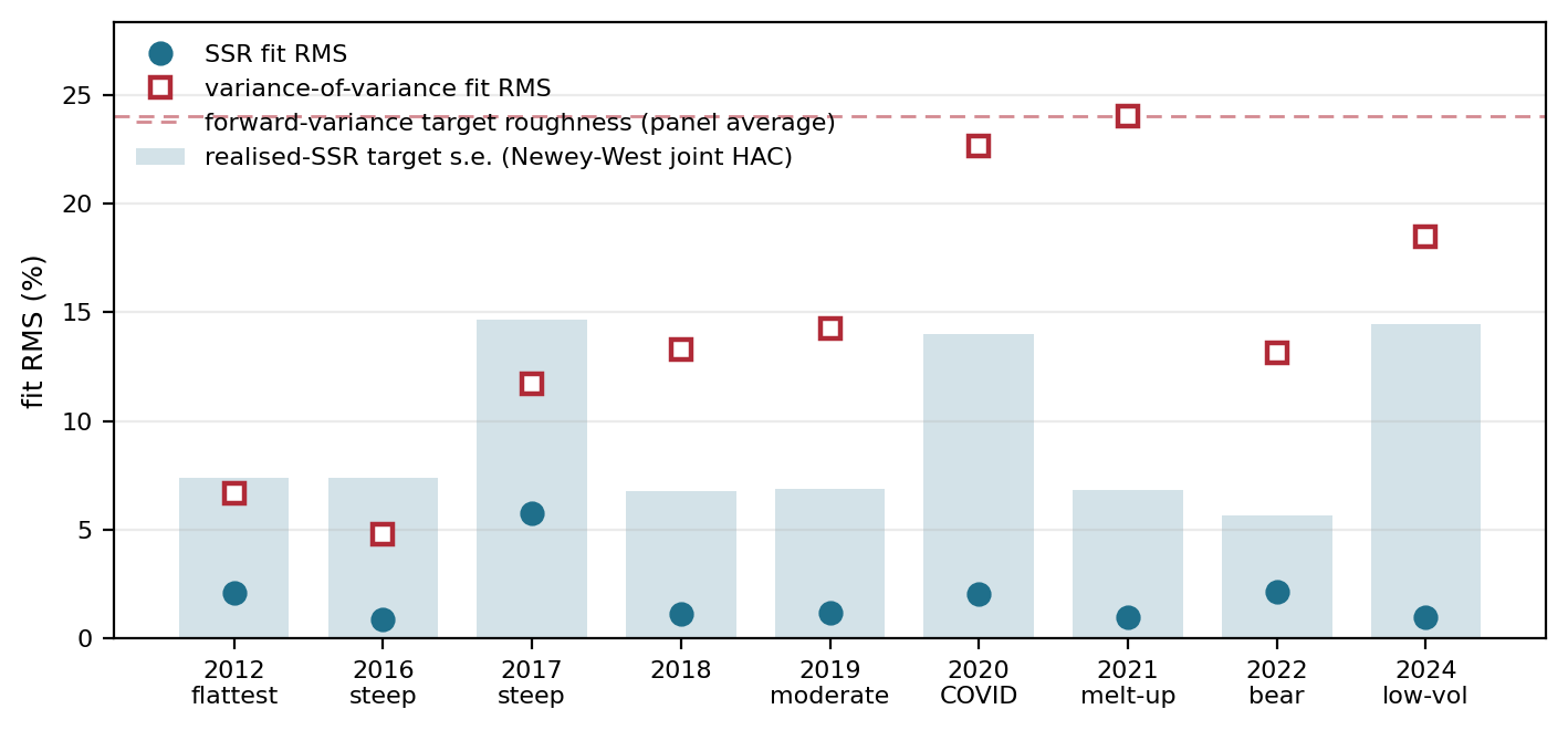
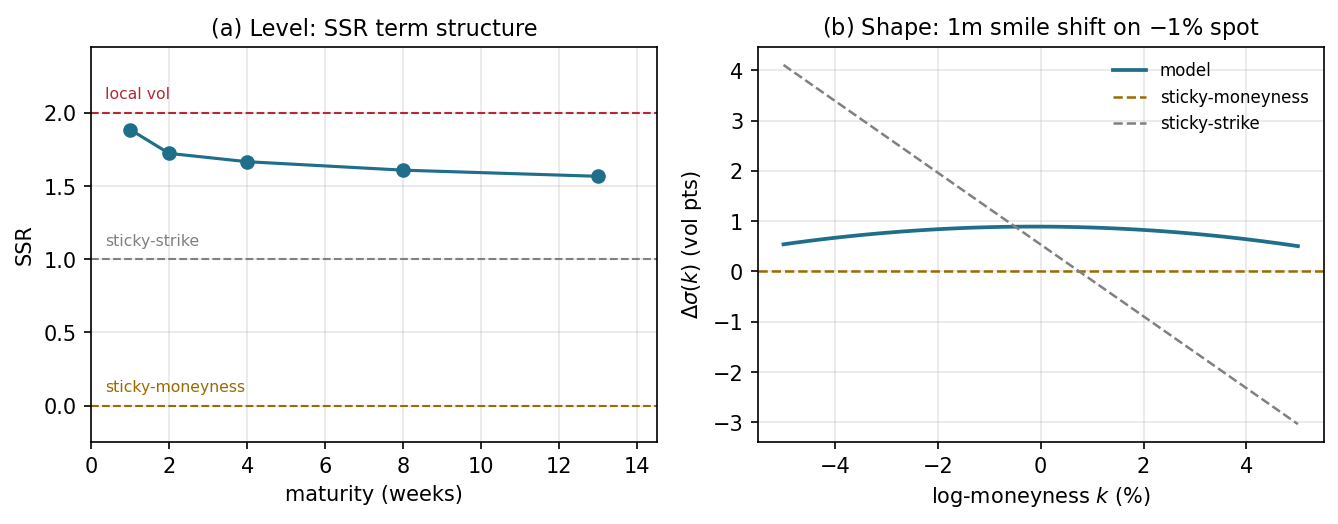
European option prices identify risk-neutral marginals but not the martingale transition law connecting them. SANOS-Evolve fixes an arbitrage-free marginal surface—supplied by the SANOS framework—and calibrates a discrete stochastic-local-volatility construction to two complementary observable readouts of leading-order at-the-money smile dynamics: the skew-stickiness ratio (SSR), a normalised measure of spot–volatility coupling and its maturity decay, and a forward-variance dispersion readout carrying the amplitude that the SSR normalisation divides out. The model combines two carried volatility timescales with a finite Gaussian-mixture return kernel. A log-sum-exp normalisation makes it a martingale by construction—exactly so before the recompression that holds the component budget flat, and measured rather than guaranteed after it—while a deterministic leverage overlay aligns the conditional variance level with the fixed marginals to leading order in the step. This yields analytic one-step finite-mixture propagation and deterministic readouts.
The two targets live under different measures, and the paper states the identification restriction linking them rather than asserting an equality. The forward-variance observation is VIX at-the-money implied volatility on SPX and a corrected realised strip off index, entering as a softly weighted reading rather than a coequal joint-calibration market. Across nine SPX regimes from 2012 to 2024 one uniform protocol places the model skew-stickiness inside every year’s sampling band (–RMS) and fits the VIX curve to –RMS; an NDX study preserves the SSR fit but exposes a two-timescale decay limit. What is identified is a class of observationally equivalent kernels, not a unique parameter vector.
Understanding how the implied-volatility smile evolves is a central problem in derivatives pricing and risk
management. A European-option surface can be fitted accurately across strikes and maturities and still
leave forward-starting prices, path-dependent exposures, and smile-aware hedges undetermined. The
reason is that vanilla prices pin down the distribution of the underlying at each maturity without pinning
down how it travels between them.
That gap has a precise statement. At each maturity , under the usual regularity and no-arbitrage
conditions, the call surface determines a risk-neutral marginal [3]
Across maturities, however, the family
constrains but does not determine the conditional transition law
Infinitely many martingale kernels carry
the same marginal chain—the observation that underwrites the model-independent bounds of martingale
optimal transport [20]. Every quantity listed above depends on which of them the market is taken to
follow, and the vanilla surface does not choose. Selecting one is a second inverse problem, layered on top of
static calibration.
Yet “smile dynamics” is not itself an observable calibration target. Before a parametric family is
imposed, the missing transition law is infinite-dimensional, and the statement that spot and volatility
move together stays qualitative until one names functionals that can both be estimated from data and
evaluated on a candidate kernel. Those functionals fix two things at once: what agreement with
observed dynamics is taken to mean, and how two otherwise admissible kernels are to be
compared.
We therefore work with two complementary leading-order at-the-money readouts. The first is the
skew-stickiness ratio, the normalised regression response of at-the-money implied volatility to a spot
return,
Its level places the smile response on the sticky map—sticky-moneyness, sticky-strike, and the
local-volatility regime above them—and its term structure measures how far that coupling persists with
maturity. Being a ratio, though, it is comparatively insensitive to the amplitude of volatility’s own motion:
to leading order in this normalisation the denominator carries the same scale as the numerator, so much of
the amplitude cancels. A forward-variance dispersion readout supplies that missing scale, observed on
SPX through the VIX at-the-money implied-volatility term structure, which is sensitive primarily to the
dispersion and persistence of future variance. The two are coupling and amplitude coordinates
rather than substitutes—each is dominated by one of them, neither is a pure measurement of
it. Together they are a parsimonious and empirically checkable description of leading-order
at-the-money dynamics—not a complete statistic for the transition law. Calibrating to them identifies
the corresponding readout-equivalence class within the chosen kernel family, and nothing
finer.
This paper takes that selection as its subject. We propose SANOS-Evolve, a discrete
stochastic-local-volatility framework that treats the missing transition kernel as the object of calibration.
An arbitrage-free marginal surface is supplied by the SANOS framework [1] and held fixed, while a
tractable two-timescale Gaussian-mixture kernel is calibrated to those two readouts. The two layers share
one representation: read as a density fit, SANOS delivers each as a finite Gaussian mixture in
log-moneyness—via Black–Scholes evaluation of its basis components, restated in Appendix A—and
propagating one through a Gaussian-mixture kernel as in (1) returns a finite mixture again. Before the
state-dependent leverage overlay the intrinsic propagation stays exactly inside the class; the overlay
retains it through the collocation and recompression of Section 3. Either way the dynamic
readouts are deterministic fixed-resolution evaluations rather than simulations. A deterministic
leverage overlay aligns the conditional variance level with the prescribed marginals, leaving the
kernel to describe the relative volatility states, their persistence, and their dependence on the
return innovation. The resulting finite-mixture construction admits explicit propagation and
deterministic dynamic readouts. In the empirical implementation the realised skew-stickiness term structure is the primary target and the forward-variance block is softly weighted beside
it.
The paper develops this identification architecture (Section 2), constructs the martingale kernel
(Section 3) and its readouts (Section 4), and evaluates it across SPX and NDX regimes and in a
smile-roll replay (Section 5); the approximation and stability results supporting the broader mixture
framework are stated where they are used and proved in Appendix B, while target construction and the
calibration protocol are collected in Appendices D–E.
1.1Kernel-first identification
Conditional on the fixed marginal surface, the transition kernel is the unknown and observed dynamic
behaviour selects it (Figure 1).
Figure 1. The identification pipeline (upper row) and the instance implemented here (lower
row). The general construction needs only a convex-ordered marginal engine, an admissible
martingale-kernel family , and a dynamic readout ; the kernel is the unknown. Two blocks
are calibrated—the coupling readout and the amplitude readout —and what they select is a
representative of a readout-equivalence class, not a unique kernel. The digital band runs the
other way: it is emitted and reported at zero loss weight (dotted), a diagnostic of the leverage
overlay rather than a target. Everything to the right of the kernel is model-implied. The lower row
instantiates each stage with the SANOS marginal engine, the two-timescale Gauss–Hermite kernel
with a Gyöngy leverage overlay, and the deterministic digital, skew-stickiness and variance-index
readouts.
The construction separates the marginal level from the relative stochastic-volatility structure.
Conditional on the carried volatility state the intrinsic return law is translation-invariant in log
spot—computationally valuable, but unable in general to connect an arbitrary prescribed marginal
pair—so a deterministic state-dependent leverage overlay supplies the local scaling the fixed surface
implies, while the intrinsic kernel keeps the dispersion, persistence and return–state dependence the
readouts identify. At finite resolution the resulting marginal compatibility is measured by the digital
residual rather than assumed.
The implemented kernel is a parsimonious realisation of that architecture: two carried persistence
timescales and a renewed within-step return branch, with martingality imposed structurally by a
log-sum-exp normalisation. Conditional on the volatility state and the branch the log-return is Gaussian,
so the transition law is a finite Gaussian mixture whose weights and moments are explicit functions of the
parameters, and one-step propagation of the intrinsic kernel is an analytic mixture update. Finite
mixtures have a long history as a tractable smile-consistent family [12]; specifying the transition law
directly rather than a driving process has an architectural analogue in Markov-functional interest-rate
models [45], which share a low-dimensional Markov driver, a deterministic functional calibration map and
an efficient implementation. That analogy is structural—what selects the kernel here is observed dynamic
behaviour.
The readout vector implements those two coordinates and carries a third block that is reported rather
than optimised. is the realised skew-stickiness term structure, read at five tenors from one week to three
months. is the forward-variance dispersion block, whose market observation is the VIX at-the-money
implied-volatility term structure on SPX and a corrected realised strip off index—related
observation operators occupying one slot, not the same quantity. Only these two enter the
objective. The third, , is a fixed digital band comparing the propagated and target marginals: a
diagnostic of the leverage overlay’s finite-resolution performance, entering the loss at zero weight.
Section 4 gives each observation operator, the measure each lives under, and the identification
assumption linking the pooled physical-measure regression to its within-regime risk-neutral
analogue.
The static layer used in the empirical implementation is SANOS [1]. It fits weights only,
over a fixed grid of Gaussian bumps in log-moneyness sharing one bandwidth, each priced by
Black–Scholes; its linear program enforces convex order. The fitted marginal is therefore itself a finite
Gaussian mixture—a smoothed grid of point masses, which the bumps become as the bandwidth
vanishes.
That representation is why this engine and not another. The marginal layer arrives in the same class
the kernel propagates, so a mixture updated by a Gaussian-mixture kernel is again a mixture, and the
local variance and its Breeden–Litzenberger density are closed forms on that same object. We retain those
marginals and replace the canonical discrete-local-volatility transition associated with them. The
architecture itself asks only for a convex-ordered marginal engine with an explicit tractable
representation—arbitrage-free surface interpolation [41] and its mixture-preserving variants [46]
supply alternatives—but it is the closure under propagation that keeps every readout a finite
sum.
1.2How existing methods select the kernel
Other constructions select the same missing law by other means. Process-first models—Heston [9], SABR [10], the Bergomi family [22, 23], rough volatility [25, 26]—specify state dynamics and derive the
kernel, so smile and smile dynamics are encoded together. Local projection draws the dynamics from the
marginals: Dupire local volatility [2] and the contemporaneous implied trees [4, 5] are the limiting case in
which the static surface determines the dynamic law—so its skew-stickiness is pinned by the static skew,
near the Doeff–Kamal value under an empirical scaling [39], while the measured SPX term structure is
materially maturity-dependent. Stochastic-local volatility[7, 8, 13] fixes a backbone and identifies a
leverage function through Gyöngy’s projection [6], by particle or learning-based schemes [14, 16], with
existence known in the regime-switching case [17]; the leverage recovers the marginal projection,
while the remaining conditional dynamics stay backbone-dependent. Transport and entropy
methods—Bass constructions [42, 44], martingale optimal transport [43, 15], martingale Schrödinger
bridges [35]—impose marginal or market-price constraints and select an admissible law by a variational or
entropic criterion.
A fourth family models the observable surface directly: market models of implied volatility posit
surface dynamics and derive the no-arbitrage drift restrictions those dynamics must satisfy [32, 33], and
recent work learns the joint dynamics of liquid option prices under no-arbitrage constraints [34]. Selecting
dynamics from observed surface behaviour is therefore not new; what differs is the object carried. Those
models evolve the surface, so static no-arbitrage is a constraint their dynamics must respect at every date,
whereas the marginals here are fixed once by a convex-ordered engine and the unknown is the kernel
between them.
In each family the smile response follows from the chosen process, projection, or optimality principle,
and the empirical consequence is measurable. Calibrating two-factor Bergomi, rough Bergomi, rough
Heston and Heston as closely as possible to the same SPX smile, [29] finds SSR term structures
that all deviate materially from the market’s, and concludes that roughness alone does not
change the joint spot–volatility dynamics enough to close the gap; [27] supplies the analytic
counterpart, a model-free expression for the SSR whose short-time limit is rather than the diffusive .
The statistic can also be targeted directly: the two-factor Quintic OU model [30] calibrates
to SPX at-the-money volatility, skew and SSR term structures, and separately to the joint
SPX–VIX smiles under a penalty holding the model SSR inside . One qualification shapes
what is claimed below: such comparisons are drawn against point estimates of a windowed
realised SSR carrying no sampling band, whereas every fit here is reported against its own
displayed precision scale, which is the target’s joint-HAC standard error at every date but one
(Appendix C).
Adjacent joint SPX–VIX calibration. Joint SPX–VIX calibration addresses a related but different inverse problem. Guyon imposes
SPX-smile, VIX-future and VIX-smile constraints and selects a minimum-relative-entropy law [37, 35];
Guo, Loeper, Oblój and Wang formulate finite SPX and VIX price constraints through semimartingale
optimal transport [36]; and Che et al. derive first-order risk perturbations around an entropically
calibrated SPX–VIX coupling, using the SSR to transmit SPX shocks to the VIX side [38].
SANOS-Evolve does not seek to reproduce a variance-index market. It fixes each underlying’s
marginal chain and calibrates a restricted explicit kernel to skew-stickiness and a softly weighted
forward-variance-dispersion readout. VIX at-the-money implied volatility supplies that observation for
SPX; off index, a corrected realised proxy built from the underlying’s own option strip fills the same slot,
and variance-index futures are not separate calibration constraints. The distinction that matters is
therefore joint cross-market calibration versus portable readout-based kernel calibration, not competing solutions to one fitting problem.
1.3Contributions and findings
The paper makes three contributions.
1.
Dynamic-readout identification of a stochastic lift. We develop a selection principle for smile dynamics: conditional on an independently fitted marginal surface, the latent transition kernel is calibrated directly to the two complementary leading-order readouts motivated above, and what it selects is a readout-equivalence class. A deterministic leverage overlay supplies the local variance level, while the kernel controls the relative stochastic-volatility states, their persistence, and their dependence on the return innovation.
2.
An explicit finite realization and approximation foundation. We construct a two-timescale Gaussian-mixture martingale kernel with structural fibrewise normalization, analytic one-step mixture propagation, and deterministic finite-sum SSR and variance-index readouts. Two propositions accompany the construction—leverage and finite-kernel stability (Proposition 2) and dynamic-readout regularity (Proposition 3)—proved in Appendix B.
3.
Cross-regime evidence and identified limits. Across nine SPX regimes from 2012 to 2024, one uniform protocol places the realised SSR term structure within every year’s HAC sampling band (– RMS) and fits the VIX ATM implied-volatility term structure to – RMS. An NDX study using own-strip and realised forward-variance observations preserves the SSR fit but exposes a steep-decay limitation in the variance-of-variance term structure. A smile-roll replay—a residual-variance proxy, not traded profit and loss—suggests that the benefit of a smile-aware adjustment is stability relative to a trailing realised regression rather than superior short-horizon forecasting; a fixed ratio performs similarly.
The baseline is an ATM-dynamics model: it targets the level response summarized by
SSR and one forward-variance distributional readout, with VIX entering as a softly weighted
observation rather than as a joint calibration target. Its diffusive finite-factor structure does not
reproduce rough scaling, and translation invariance excludes spot-level dependence of conditional
smile shape beyond the latent-regime channel. Section 6 evaluates those limits against the
evidence.
2Identification architecture and guarantees
The marginal engine supplies an arbitrage-free spot law at every listed maturity. The dynamic unknown is
a transition kernel on a lifted spot–volatility state, whose role is not to refit the vanilla surface but to
select a conditional coupling whose observable dynamics agree with the chosen readouts. This section
defines those objects and separates the ideal admissible problem from the finite-resolution construction used in calibration.
2.1The identification problem
Fix a pricing date and maturities with forwards and discount factors , and work in log-moneyness . Four
objects.
A fixed marginal chain. An external convex procedure returns arbitrage-free spot laws , increasing in
convex order, with an explicit finite mixture representation. They are fixed once and are not re-fitted
when the dynamic targets change.
A lifted source law. The kernel acts on a lifted state carrying a latent volatility regime, with law
whose spot projection is the engine’s output, . What is transported from one maturity to the next is ; the
engine pins only its projection. A spot marginal cannot be pushed through a kernel whose source carries a
latent volatility state.
The ideal family, and the implemented object. The ideal family is the set of Markov kernels on the
lifted state that are positive, normalised, martingale in the forward-normalised spot on every fibre,
and—together with a deterministic leverage overlay—propagate to . The implementation does
not sit in it, so the implemented object is not a kernel at all. It is a law-evolution pipeline :
an overlaid finite kernel applied to a mixture, followed by the recompression projection of
Section 3.4, which maps laws to laws and is not a Markov kernel. The pipeline is indexed
by , the box of Section 5. Section 2.2 says what retains of admissibility and what it does
not.
A dynamic readout. A map returning the finite vector of quantities the calibration actually measures,
defined on a kernel or on a pipeline alike. Identification is the inverse problem
in the ideal statement, over
kernels, and
as implemented—over parameters indexing the pipeline, and over the calibrated blocks only,
since carries zero weight. Every fitted object in this paper solves (4); (3) is the problem it approximates.
Here is the observed targets and a fixed weighting; Section 4 writes out in full. Figure 1 sets this
architecture beside the instance implemented here and against the standing answers to the selection
question.
2.2Ideal and finite-resolution admissibility
Definition 1 (Admissible kernel) .Fix the lifted source law of Section 2and the target spot marginal . A
Markov kernel on the lifted state is admissible if
The conditions are, in order: positivity,
normalisation, the (forward-normalised) martingale property, and exact propagation of the spot
marginal.
Definition 2 (Finite-feature marginal compatibility) .The production chain is not an element of , and
we do not claim membership of a Wasserstein ball around it. Two of the four conditions in (5) hold
outright—positivity and normalisation—and the martingale condition holds in the weakened form
with the -algebra the implementation conditions on (the component index and the price abscissa of (23)) and
before the recompression projection of Section 3.4, which preserves mass and the unconditional forward
only. The fourth condition, exact propagation of the spot marginal, is replaced not by a metric bound but
by a finite-feature discrepancy: the seven-threshold digital vector of Section 4.2, together with
the call-price and implied-volatility residuals at the quoted strikes. These are what Section 5reports.
The natural metric would be on the forward-normalised marginals, which in one dimension is
the second
equality because for undiscounted calls—so is the total variation across strikes of the call-price difference.
A finite set of quoted strikes does not resolve that total variation, so we report the discrepancy we can
measure and make no claim about .
Theorem 1 (No static arbitrage) .Let be probability measures on with . Assume their
forward-normalised laws are increasing in convex order, . If are admissible (each ), then for any
initial lifted law with , the lifted chain satisfies for every , and is a martingale in the lifted
filtration—so the discounted underlying is a martingale with one-dimensional marginals exactly .
The induced call surface is then free of strike (butterfly) and calendar static arbitrage. Moreover for every .
Proof sketch.Strike no-arbitrage. For each , is a probability measure with ; hence is convex and
non-increasing in with the correct bounds, which is equivalent to absence of butterfly arbitrage [3].
Martingale and marginals. Admissibility gives for every lifted state , so is a martingale in
the lifted filtration. It also gives ; propagation happens on the lifted law, , and only its projection
is pinned. Starting from , induction gives for all , so the spot marginals are exactly and the
discounted underlying is a martingale.
Calendar no-arbitrage. A martingale transition implies, by conditional Jensen, that the
forward-normalised marginals are increasing in convex order, , which is equivalent to absence of
calendar arbitrage for the call surface.
Existence. By Strassen’s theorem [19, 20] a martingale kernel on the forward-normalised spot
coordinate with exists iff , and SANOS enforces that convex order across maturities. Strassen returns a
spot object, so it must be lifted before it is an element of . Disintegrate the coupling as , let the transition
ignore the current latent label, and attach any probability law for the next one: ∎
This is non-negative and
normalised; it is fibrewise a martingale, since for every ; and for any projecting to , . Hence
.
The content is that the no-arbitrage claim attaches to the admissible set, and that the set is nonempty
precisely because SANOS delivers marginals in convex order (Strassen). The discrete-local-volatility
transition associated with the SANOS parameterisation [1] becomes an element of once embedded
in the lifted state—for instance with latent labels drawn independently of the return—and
it is the rigid element the introduction set out to replace. The two calibrated readouts of
Section 4select a different, controllable element of in the ideal statement, and they never replace
the set. What is fitted is not that element: the production pipeline is not in at all, since
it satisfies the martingale condition at its own numerical state and before recompression,
and replaces exact marginal propagation by the finite-feature discrepancy of Definition 2.
is the ideal object the construction targets, not a set the implementation is claimed to sit
in.
One question remains before any particular kernel is written down: is the class we are about to restrict
to rich enough to be worth restricting? The useful form of that question is not density among admissible
martingale kernels but whether the family’s readout image covers the behaviour the market shows—a
finite-dimensional question, answered by the attainable-range experiment of Section 5.1 and
the nine-regime panel of Section 5.3. Table 1 records which layer every later claim attaches
to.
2.3Structural guarantees and approximation layers
Each layer of the construction carries a property that holds exactly, by structure, and a separate element
whose accuracy is finite. Table 1 grades them, and every later use of “exact” names the row it belongs
to.
Table 1. Structural guarantees and finite-resolution layers. The middle column holds exactly by
construction; the right column is measured and reported.
the branch rule is a fixed quadrature, exact in its own moments
Gaussian closure: the marginal law is a finite mixture, propagated by its moments
Marginal compatibility
nothing structural: the overlay targets it, no limit theorem is claimed
finite-resolution digital discrepancy
Readouts
deterministic fixed-resolution evaluation of the implemented finite functional
central difference, Newton inversion, quadrature and interpolation
What the construction avoids, relative to classical stochastic-local volatility, is the continuous-time
leverage fixed point.
3A finite martingale realization
We now construct one tractable member of the admissible architecture. The design has four steps. A finite
branch kernel represents the joint return–state transition; a two-timescale coefficient map supplies
persistence and leverage; a structural normalization enforces martingality; and a deterministic
local-variance overlay aligns the conditional variance level with the fixed marginal surface. The resulting
kernel remains explicit enough to propagate as a finite Gaussian mixture.
3.1A finite martingale kernel
The state is the lifted pair of Section 2, written concretely as
with log-spot and two continuous latent
volatility factors, each standardised to unit stationary variance. The class of kernels we work in is
a finite
mixture over a within-step branch index of Gaussian return increments, each branch carrying its own
Gaussian transition of the two factors. Three properties of (10) do the structural work, and the rest of
the paper leans on them repeatedly.
Translation invariance of the intrinsic return law. The spot enters only as the additive centre of the
Gaussian, so the conditional return law—and hence the conditional smile in moneyness—depends on the
factor pair alone, not on the spot level. This is what makes the intrinsic propagation an exact mixture
map, before the marginal overlay reintroduces a -dependence (Section 3.4), and the dynamic readouts
deterministic finite sums (Section 4).
The branch index mediates return–factor dependence. A common appears in both the Gaussian mean
and the factor transition , so the joint law of return and next factor state is not a product of its marginals.
This is precisely the dependence that leverage and skew-stickiness measure, and it is why an
approximation theorem for this class must control the joint conditional law rather than the two
conditional marginals separately (Appendix B).
Gaussian destination factor law. Each is Gaussian, so a law carried as a Gaussian mixture in maps to
another one and every readout reduces to a finite quadrature sum—not to a sum over a latent alphabet, of
which there is none.
The two carried factors and the within-step branch play different roles, and the distinction matters
throughout:
Table 2. Roles of the two carried factors and the within-step branch. Sans-serif name them. Only
the branch carries a node count, : the two persistent factors are continuous and are propagated
as Gaussian moments rather than on abscissas (Section 3.4), so they have no node count of their
own.
Index
Persisted across steps?
Economic role
yes (continuous)
fast volatility factor; the decaying short end of the skew-stickiness term structure
yes (continuous)
slow volatility factor; the sustained long-end floor
no (renewed each step)
within-step return branch; carries the instantaneous skew and the return–factor coupling
Spot marginal versus lifted law. The kernel acts on the joint state, so its one-step law is a lifted joint , whereas the marginal engine
supplies only the spot marginal . The first maturity is lifted with the stationary bivariate factor law
of (17); thereafter the joint is carried by the propagation. Throughout, abbreviates the match of spot
marginals after propagation of the lifted law, .
Equation (10) admits unrestricted weights, drifts and variances; the implementation below restricts
them to an eight-coefficient image, seven of them fitted. Two scope points belong here rather than in the
appendix. Appendix B establishes stability and readout continuity for the overlaid finite kernel, and no
approximation-theoretic claim is made for the family: what that image reaches is answered by
measurement (Sections 5.1 and 5.4), not by a density theorem. And the two operations the
production chain performs at every step—evaluating the leverage overlay by collocation at finitely
many price abscissas (Section 3.3), and recompressing the propagated mixture back to a fixed
component budget (Section 3.4)—appear in no result of that appendix, which is stated throughout
at a fixed numerical pattern (Remark 1). Their effect is measured (Section 5) rather than
bounded.
3.2The two-timescale specialization
The volatility state is a baseline plus a fast and a slow mean-reverting factor, the two-factor Bergomi
picture [22, 23]. Conditional on that state the one-step log-return is Gaussian, but its mean and variance
are functions of a continuous latent state, so the kernel is an integral over the factors rather than a finite
mixture. The remedy is quadrature— applied to the factors’ effect on the log-variance, not to
the factors themselves, which stay continuous throughout. An -point Gauss–Hermite rule
represents by nodes and weights reproducing its moments through order ,
so replacing
each continuous latent quantity by its nodes turns the integral into a finite sum, each node a
volatility scenario. The nodes, base log-weights and within-step weights are fixed quadrature
constants.
Eight structural knobs determine every coefficient in (10); the level is a ninth coefficient but is solved
rather than fitted, from the reference-variance condition (18) below.
Each carried factor is a standardised Gaussian AR(1),
with standard normal innovations, so each has
unit stationary variance and is exactly the one-step autocorrelation, . This is the continuous-shock
idealisation. Production replaces the branch part of each innovation by the finite Gauss–Hermite rule
of (11): conditional on a branch the factor step is Gaussian, but marginally the carried law is a finite
Gaussian mixture, and every “Gaussian” statement below—the bivariate stationary law of (17), the -step
law of (40)—is that idealisation, realised by matching moments and closing the recursion in the Gaussian
family. The closure is a quadrature approximation, not an identity, and its error is not measured here: the
refinement study of Section 5.2 varies node counts and the recompression budget, which is a different
comparison. Quantifying the closure would mean propagating the full mixture against the
moment-closed recursion, and we do not report it. The leverage is a correlation between those
innovations and the branch variable that drives the return,
leaving each factor an idiosyncratic
innovation variance . This is the return–factor channel of (10): a branch carrying a large negative return also tilts both factors, and it does so through the innovation rather than through
log-spot.
The two factors enter the return law only through the scalar combination , so the branch variance and
the within-step skew tilt are
the drift of (10) following from by the martingale lock (19). Only is integrated by quadrature, at
nodes; the factors themselves are never placed on abscissas. One derived quantity recurs throughout: the
full one-step increment variance at a factor state,
the law of total variance applied across branches—the
within-branch term plus the mean spread the skew tilt creates. It is what the level condition, the leverage
overlay and the forward-variance readout all measure.
Under (12)–(13) the stationary factor law is bivariate normal with unit marginals and correlation
writing for the innovation scales. The only channel coupling the two factors is their shared leverage on
the return branch: if either vanishes they are stationarily independent. The level is then fixed by requiring
the stationary expected one-step variance to match the reference,
which determines and removes it from
the fitted vector.
The parameters separate by role: set the spread of the log-variance across the two factors and its
within-step dispersion; the return skew; the persistence; and the return–factor dependence, the
innovation leverages. A down move tilts the factors toward higher volatility through . Because the leverage
enters the innovation around a fixed stationary target rather than shifting that target, the equilibrium
volatility is not a deterministic function of spot: this is genuine stochastic volatility, and the kernel stays
translation-invariant in .
Since is an autocorrelation it carries an effective rate directly, through the one-step half-life , and
needs no separate interpretation. Across the nine SPX fits of Section 5.3 the ordering holds at every date,
with median half-lives of weeks fast and weeks slow, so the two timescales the construction posits are the
two the calibration finds.
The finite approximation is not a discretisation of the two persistent factors. They are carried
continuously—each step propagates their means and covariance, and the state passed between steps is per
component—so what is finite is the quadrature that integrates their combined effect on the
log-variance, the within-step branch count , the price sub-abscissas, and the recompression budget.
Production values and the measured readout sensitivity are reported with the empirical protocol in
Section 5.
3.3Structural martingality and the marginal overlay
Martingality is enforced twice: once on the intrinsic kernel, and again after the market-level overlay that
rescales its variance. The first is stated for the ideal construction, at a fixed latent state; the second is
what the implementation performs, and it conditions on the numerical state instead. The difference is
spelled out below and is not cosmetic.
Stage 1: the intrinsic kernel (ideal). The within-step drift is locked to the forward on every fibre—the kernel’s conditional law at a fixed
state , with the continuous factor pair. Writing for the skew tilt of (14), so that the raw mean is ,
subtract the per-fibre constant
so that exactly at a realised (Proposition 4). The shift is a single
per-fibre constant, independent of , stable and differentiable, and it preserves the relative branch tilts that carry the leverage and the skew-stickiness.
Stage 2: the market-level overlay. A translation-invariant kernel cannot, on its own, carry a prescribed marginal chain: its
unleveraged propagation has convolution form , which connects only marginal pairs admitting a
common increment-law representation. Matching is restored by one deterministic ingredient, a
leverage overlay that rescales the conditional variance. Writing the increment as a local scale
times a unit stochastic-volatility factor,
with of (16): the first two factors are the target
decomposition, exact in the continuous-time limit, and is what the weekly step leaves at a fixed
latent state. The implementation does not condition there, so a second remainder —same
algebra, coarser conditioning—appears at (24) below and is the one measured; the two are not
the same number, and only is reported. Taking alone mis-scales the leverage by at the
calibrated . The overlay itself is the finite-kernel analogue of the stochastic-local-volatility
leverage relation,
with read from the fixed marginals: a closed-form Gaussian-mixture call, a
Breeden–Litzenberger density, and a calendar finite difference. That difference is well posed only on a
convex-ordered surface, which is what the constraint in Algorithm 1 is for; the overlay inherits that
hypothesis from the marginal engine (Assumption 1). Rescaling the variance changes , so the drift
must be re-locked after the overlay rather than carried over. Writing , the overlay scales
the
variances by and the skew tilt by , and then re-locks. Two things follow, and only the first is
exact.
The forward is restored exactly, at the state the implementation carries. The production lock is taken
over the branches and the component’s own factor quadrature together,
with the component’s factor
nodes and their weights (Section 3.4), so that identically (Proposition 5). That is martingality at the
numerical information state—the component index and the price abscissa—which is the filtration the
propagation actually carries. It is not the same as martingality conditional on a realised : the two coincide
only where the component’s factor law is degenerate.
The conditional variance is matched to leading order, not exactly. Because variances scale by while the
tilt scales by , the branch dispersion of the drift does not scale as . At the state the implementation
conditions on—the component and the price abscissa of (23)—
both terms vanishing at , with the
moments taken over the joint factor-node/branch law that the lock normalises over. The
same algebra at a fixed gives the same expression with branch-only moments, but that is
a finer information set than the implementation uses and understates the discrepancy by
roughly a factor of two: and are different quantities and only the latter is reported. Since
and the covariance term dominates and both remainders are , so the relative error is —at a
weekly step that is not automatically negligible, and Section 5.2 measures it rather than
bounding it. Equation (21) is therefore the continuous-time relation the weekly construction
targets, and the finite step realises it to leading order. The re-lock of (23) shifts every branch by
one constant, so it restores the forward without touching . The complete per-step pipeline is
The division of labour. This is the decoupling that organises the paper, and it is stated here once, with the moment it applies
to named. The marginal engine determines the local variance level; the intrinsic kernel determines the
relative regime dispersion and the return–regime dependence. The overlay is a variance rescaling, so what
it carries is the second moment: the per-step enforcement is (21) followed by the martingale re-lock (23), which fixes a variance and a mean and constrains nothing beyond them. The propagated
skew is therefore not carried by the overlay but generated by the kernel, through and the
innovation leverages, and Section 5.3 measures how far short of the target marginal’s skew it
falls. The -average of (20) equals up to the finite-step remainder of (24), so the level is the
leverage’s responsibility and the kernel enters only through the unit-mean ratio . Positivity and
normalisation are structural in the coefficient map and martingality holds at the numerical state
before recompression; marginal compatibility is the overlay’s; and calibration therefore fits only
dynamic parameters. The kernel’s own level nearly divides out of and is reset by , leaving it
close to inert; what survives is the relative structure of the factor state—the spread and,
through (12) and (13), the autocorrelations and the innovation leverages—which is exactly what
the two calibrated readouts interrogate jointly: the leverages and the spread set the coupling
that measures, the spread and the autocorrelations set the amplitude and persistence that
measures.
The overlay is a composition of three maps—conditional variance, leverage ratio, overlaid kernel—and
each must be stable for approximation of a target-compatible limit to transfer to the finite-mixture
implementation.
Proposition 2 (Leverage and finite-kernel stability) .Let the spot-conditional variances converge
in , —which Assumption 1(iv) supplies from convergence of the source laws, and which we assume
rather than derive, since conditional expectations are not Lipschitz in adapted topologies [21]without further structure. Let the regularised local-variance input converge, , and the coefficient
vectors converge, . Then, on the compact nondegenerate region of Appendix B, the leverage ratio ,
and the overlaid finite kernel all converge, the last in integrated conditional Wasserstein distance.
The hypothesis on is not decorative: the bound of Proposition 6is , so a coefficient sequence that
does not settle gives a kernel sequence that does not either, however well behaved the source laws
and the local variance are.
Proof idea. Stability of the conditional mean is not derived here—it is Assumption 1(iv), for the reason
given there. Granting it, the ratio is stable because is bounded away from zero on the nondegenerate
region; and the overlaid kernel depends on through locally Lipschitz coefficient maps, a locally Lipschitz
log-sum-exp re-lock, and a Gaussian-mixture bound. The proof is Proposition 6, at the fixed numerical
pattern stated there.
Here is the spot-conditional average of the unit factor, distinct from the stationary and tilted only by
the spot–volatility correlation. For marginal matching—each step re-seeded from the target law—it is
close to and the residual is discretisation rather than bias. Under multi-step concatenation from a fixed
spot (forward densities, hedging) it is not: the negative leverage tilt correlates high- regimes with low , so
on SPX, and ignoring it under-reads the accumulated ATM level by in volatility over a
multi-month chain. The full spot-conditional correction of (21) is therefore retained for absolute-level
outputs.
3.4Propagation and component control
One-step propagation of the intrinsic kernel is exact. Translation invariance means the discretised kernel adds, conditional on a regime, a fixed Gaussian
increment—constant in the integration variable—and fixed Gaussians convolve in closed form:
A law
carried per component as a Gaussian in therefore propagates to a finite mixture of such Gaussians,
where are the Gauss–Hermite weights integrating that component’s own log-variance combination
—itself Gaussian, since the component is—and is the affine factor update of (12)–(13), with and the
branch-dependent mean shift carrying the leverage. The coefficient variability lives entirely in the
outer sum over and never inside a convolution, so propagation of the intrinsic kernel is an
exact finite Gaussian-mixture update, needing no state-space integration, PDE solve or Monte
Carlo.
The production chain is not that object, and the difference should not be collapsed. The leverage
overlay of Section 3.3 scales the branch variances by , and that -dependence is exactly what
breaks (25): fixed Gaussians convolve, -dependent ones do not. Each overlaid step is therefore closed
by a first-order collocation in rather than by the identity above. What survives exactly is
structural—positivity and normalisation at every state and parameter value, and martingality
at the numerical state (23)—while the local-variance match carries the remainder (24) and
marginal propagation is approximate; Table 1 grades which is which. The collocation residual is
moreover a property of the overlay rather than of the component budget: the Gyöngy match
is re-imposed at every step, so this is a first-order approximation error and not a quantity
that refining the recompression drives to zero. (A Monte-Carlo cross-check showed the same
collocation biases the multi-step skew-stickiness when it is applied to the intrinsic branch law
instead.)
Why the component count must be controlled. Equation (26) multiplies the component count by at each step, where is the quadrature over the
combined factor state and the price sub-abscissas of the leverage evaluation, so composing over
steps—needed for forward densities, exotics and intermediate maturities—would leave components. A
single kernel application needs no reduction; concatenation does.
Recompression, and what it does not preserve. Each composed step therefore ends with a deterministic reduction that holds the budget flat: bands on
the two factor means and then on the price mean, and within each cell a match of mass,
mean and variance. It is a law-level projection, not a kernel operation, and the distinction
matters. A cell merges descendants originating in different source states, and the re-lock that
follows is a single scalar per chain, chosen so that the reduced mixture’s forward equals the
pre-reduction mixture’s. What the projection preserves is therefore mass and the unconditional
forward; it does not preserve the forward conditional on each preceding numerical state, and the
reduced object is consequently not itself a martingale kernel. We therefore claim no Strassen or convex-order property along the recompressed chain: exact martingality is a statement
about the pre-projection kernel (23) only, and what the chain carries past the projection is
monitored rather than guaranteed. Restoring the pathwise statement would need conditional
recompression—a per-source-cell re-lock—which the production path does not perform. Multi-step
composition therefore stays tractable as an exact mixture update followed by a deterministic
reduced-mixture approximation whose law and martingale residuals are measured and reported. The
per-step pipeline is propagate recompress (budget and global re-lock) leverage re-lock; the
recompression is the projection step. The reduction is never applied across the carried factor
bands.
Intermediate maturities. Because the carried factors are Ornstein–Uhlenbeck, the latent transition operators form a semigroup,
with mean-reversion rate ; the overlaid and recompressed production chain does not. Writing
the latent log-variance as separates a time-inhomogeneous forward-variance level from a
time-homogeneous generator, so one interpolates the one-dimensional curve and constructs
intermediate kernels by evaluation, with no matching optimisation. The carried volatility state is
what makes the construction compose at all; a spot-only kernel, marginalising the volatility
state at the intermediate step, does not, which is why a memoryless kernel needs a matching
optimisation.
3.5Summary of the construction
Table 3. What each structural feature of the construction delivers.
Property
Mechanism
positivity and normalisation
mixture weights and the softmax branch rule
martingality at the numerical state
log-sum-exp lock (23) over branches and factor quadrature
Section 1 motivates and as complementary coupling and amplitude readouts of leading-order
at-the-money dynamics. This section is the formal counterpart: it defines their observation operators,
names the measure each lives under, states the calibration map, and gives the equivalence that map
induces. One point carries over and is worth stating once as a design principle rather than a claim—the
readout is not a summary of the kernel but the topology in which it is identified, so a family is rich
enough, and an approximation good enough, only relative to the functionals one intends to read off
it.
4.1The identification map
Table 4. What each readout block observes, under which measure, and which part of the kernel it
principally constrains. The attribution is a statement about which coordinates each block is most
sensitive to, not a partition: both calibrated blocks move with most of , as Table 12 shows.
Block
Observation
Measure
Kernel feature primarily constrained
Baseline role
marginal digitals
compatibility of the leverage overlay
diagnostic
realised skew-stickiness term structure
target, analogue
return–factor leverage and its maturity decay
active
VIX ATM implied vol (SPX), realised strip (NDX)
/
forward-variance persistence and dispersion
active, softly weighted
The calibration reads these three blocks and optimises two, so two readout vectors have to be kept
apart,
the first what the objective sees, the second what is reported. Exact equivalence is a statement
about the calibrated pair alone,
an idealisation no fit attains. What a fit delivers is membership of a
production tolerance class, stated on the pipeline and with the two blocks kept apart because their
tolerances are not the same kind of quantity:
Only carries a sampling-error reading: it is set by the
skew-stickiness target’s estimated standard error. The forward-variance target is a single-day read with
no sampling band, so is a chosen calibration tolerance—the discrepancy we are willing to leave—and
nothing about it is statistical. The weightings are the corresponding diagonal blocks of the introduced
below. Every downstream identification claim is a claim about (28); densities and exotic prices are
computed from one representative of it and remain representative-specific. Write for the free
parameters, in production: the eight structural coefficients of Section 3 less , which is pinned,
and less the level , which is not a coefficient of at all but solved from by the level match
of Section 3.3. The three blocks are read on grids that the design fixes but the model does
not: a set of log-moneyness thresholds and a set of tenors, both stepped at , and a set of
forward-variance expiries. The readout vector is then
Only the last two enter the loss. The instance realises the production problem (4) with a diagonal
that vanishes on the block and normalises the surviving residuals by their own targets, plus one term
outside that form—a ridge on rather than on the readout—so the objective is best given explicitly. With
targets , stage anchor , per-tenor skew-stickiness weights normalised to , ridge weights and a floor , the
residual vector is
and the objective is its least-squares cost,
minimised over the box . The grids, the
weights and the box are design choices of the empirical study and are given with it in Section 5; the
factor is the least-squares convention, carried so that the multi-start costs quoted in Appendix E are on
the scale of (34).
Four features of (34) are choices rather than conventions. Residuals are relative: a given percentage
miss counts the same at every tenor, though the levels differ by an order of magnitude across . The
forward-variance block is normalised by its own length: the factor fixes that block’s aggregate weight at
whatever happens to be, so the cross-underlying comparison of Section 5.5 is like-for-like. The digital
block is absent, not merely down-weighted (Section 4.2). The ridge is not a target: it penalises
displacement from the stage anchor rather than misfit to data, scaled to each coordinate’s own
anchor value, and tames the railing the loosely identified directions would otherwise produce
(Appendix E).
Two counting conditions follow, and they constrain the design rather than the model. Only the and
blocks carry observations, so the data-bearing residuals number and nominal determinacy requires ; the
ridge adds further residuals, but those are regularisation rather than observation, and can only make the
optimiser well-posed on one. Identifiability asks more than counting. The parameters separate by role
(Section 3), and so does the evidence: the skew-stickiness term structure is the primary evidence for
the leverages and persistence loadings, the forward-variance term structure for the regime
spreads. Since the kernel carries two timescales, the curve is essentially a two-rate decay—a
short-tenor level, two rates and a relative amplitude—so must both be large enough to resolve four
shape degrees of freedom and span both timescales. A grid confined to tenors short relative
to steps leaves the slow factor constrained only through the ridge, however many points it
contains.
4.2Marginal compatibility
For a propagated mixture the survival probability at threshold is the finite sum , evaluated on the grid
against the interpolated target marginal at the corresponding maturity. The resulting survival
probabilities per maturity report what the leverage overlay of Section 3.3 does and does not achieve at
finite resolution; the grid used here is given in Section 5.2.
This block carries zero weight in the baseline fits: it belongs in the reported readout vector but not in
the optimised loss, and serves as an acceptance readout. A configuration with a positive digital weight is
used for the decoupling experiment of Section 5, where up-weighting degrades the dynamic fit by more
than an order of magnitude—which is itself the evidence that the statics and dynamics are separately
controlled.
4.3Skew-stickiness: a within-regime risk-neutral analogue
Three distinct objects are called “SSR” in this literature. We name them before computing
anything.
Table 5. The three skew-stickiness objects. Every occurrence of “SSR” in this paper names one of
these three.
Object
Where it lives
Role here
Empirical pooled realised-regression
Calendar-time panel under , no conditioning on the latent state
The calibration target.
Instantaneous / leading-order
Continuous-time asymptotics
Analytic interpretation, limiting values, and the hedge formula. Never a fitted quantity.
The implemented discrete kernel, stationary regime law, under
The fitted model readout. “Exact” scopes the evaluation of this functional, not equality with the pooled target.
The empirical target is the pooled regression , estimated on the calendar panel with a single intercept; the
latent volatility state is neither observed nor conditioned on. The empirical and model statistics
measure the same economic channel but are not identical functionals: the former is a pooled
physical-measure regression, the latter a stationary average of within-regime risk-neutral covariance and
variance. The calibration imposes
as an identifying modelling restriction, not as an equality of
functionals.
The two channels. The sums below run over the nodes of the stationary quadrature of the bivariate factor law (17), with
the corresponding Gaussian-copula weights. They are quadrature nodes of a continuous law, not states of
a finite alphabet: the construction of Section 3 has none. For each such node and maturity the
routine precomputes the propagated at-the-money volatility on the fixed factor–spot grid, its
slope , the leveraged branch means and variances , the branch weights , the stationary node
weights , and the Gauss–Hermite nodes and normalised weights . With realised returns and ,
the factors take their own AR(1) step,
with a further Gauss–Hermite rule, applied once
per factor because the innovations are independent given the shared branch . The one-step
at-the-money volatility change is then
the first term read off the precomputed surface by trilinear
interpolation in the two factor coordinates and the spot shift. It carries both channels: the surface
channel, through evaluation at the realised return, and the factor channel, through (35), which
moves which slice of the surface is read. No transition matrix between regimes appears: the
factor update is the continuous one of (12), and only the surface lookup is discretised. The
readout is the finite sum
normalised by the model’s own return variance and average skew,
How far apart are the two functionals? Both the numerator and denominator of (37) centre within each regime, so by the total-covariance and
total-variance identities they differ from the pooled statistic by the between-regime terms
and . Two independent measurements bound the gap. Model side: at the calibrated kernels –
and –, so global re-centring would move by at most . Data side: partitioning the empirical
panel by an observable proxy for the volatility state (the lagged one-month at-the-money
volatility), the between-state share of the covariance reaches in terciles and in quintiles, moving
the empirical by a median and at most over –, at both resolutions inside the sampling
band of Appendix C. Neither addresses the measure: the model is a -martingale whose only
regime-dependent mean return is the Jensen correction, whereas the pooled empirical between-state
terms can carry physical drift and variance-risk premium, and it is the leading-order invariance of
quadratic covariation that licenses comparing the within-state channels. That protection does not
extend to the higher-moment forward-variance channel, which governs the off-index results of
Section 5.
What the ratio means for a delta. The instantaneous object fixes the convention the values in this paper are quoted in. For a spot–volatility response coefficient and skew ,
folds the level-induced move of the at-the-money volatility
into the Black delta, with in units: is the no-roll reference and the variance-minimising choice is . For a
fixed-strike option the smile-roll term shifts this by one unit, giving , whence sticky-strike is [11]
and sticky-moneyness —the reference values against which Section 5.6 places the calibrated
kernel.
4.4Forward-variance information
As Section 1 sets out, the skew-stickiness block constrains coupling but its normalisation divides out most
of volatility’s own amplitude. This block reads the forward-variance distribution directly; on SPX its
market observation is the VIX at-the-money implied-volatility term structure, entering as a softly
weighted reading rather than as a jointly calibrated market—the object of the joint SPX–VIX
literature [37, 36, 38].
Because the carried factors are the Gaussian AR(1) pair of (12), the -step law of from any Gaussian
state today is available in closed form, with no transition matrix and no matrix power:
the unit
stationary variances of (12) supplying the constants. The cross term is the shared branch shock
accumulating over steps: and load on the same , so the two factors do not decouple, and
setting to zero would make their innovations independent while each stayed correlated with the
return. The thirty-day forward volatility is the window average of the one-step increment
variance, normalised by its stationary value so that carries the level:
with the full one-step
increment variance (16) and that same functional on the stationary factor law—the normalisation
of (18), so that returns on the stationary state by construction. Each term is evaluated by the
combined-factor quadrature of (14), since depends on only through , itself Gaussian with mean and
variance . Today’s state is a state choice rather than a parameter: the fast factor starts at
its mean and the slow level is bisected so that reproduces the observed spot index, under
no_grad and therefore outside the optimisation. That consumes one observation—the spot
variance index on SPX, the own-strip thirty-day variance-swap rate off it—which is spent on the
state and is not among the residuals counted in Section 5.2. At the option expiry, steps out,
the readout needs the law of , and the propagation of Section 3.4 supplies it: each surviving
component carries a weight , a log-price law , and a conditional factor law whose moments
are (40) run from that component’s own state. The factor is realised at the expiry, so the index
value there is at Gauss–Hermite nodes of : the residual variance is expanded, not passed
back into (41), which would turn genuine dispersion of the index into a convexity correction
on its mean. The leverage enters here as well—instantaneous variance is , so the thirty-day
rate carries too—read across the component’s own log-price nodes . Production reads it as a
root-mean-square over the variance window rather than at one slice,
normalised to unit weighted mean,
because instantaneous variance is and the index averages it over : what multiplies is the
RMS across those slices, and consecutive tenors then share of them instead of inheriting
the ladder’s per-week jumps. With the product of the four weights,
and the at-the-money
Black inversion is closed form, . Neither choice is cosmetic. A readout that drops levers the
skew-stickiness block but not this one, so the two blocks would then read different models. And
when the branch shock does not move components at all—every bit of factor uncertainty
sits inside —so folding in as convexity would report exactly no dispersion for a model with
unchanged . The market counterpart estimates the variance-index forward from a put–call
parity regression over central strikes and reads the out-of-the-money smile at that forward, so
the calibrated number is an at-the-money implied volatility rather than a generic dispersion parameter.
One qualification belongs with this block: it imposes unconditional forward-variance consistency only.
The conditional identity a genuine joint calibration would require is exactly what reading rather than
jointly fitting forgoes.
Portability. That weaker formulation is what makes the readout portable. The model side of the block does not
change with the underlying: it is (43) in every case, an at-the-money implied volatility read off the
kernel’s own forward-variance law. What changes is the observation that fills the target slot. Where a
liquid variance-index option market exists—among the underlyings here, SPX—that observation is the
market counterpart of (43) term for term. NDX has no such market, so the target is the realised
volatility of a constant-maturity variance-swap strip built from the underlying’s own options
(Appendix D, equation (51)). The two observation operators occupy the same slot in with the
same identification role and different measure content, so off index a residual in that block
carries the operator mismatch as well as any kernel error. The consequences are taken up in
Section 5.
4.5Parameter roles and identifiability
Table 6. Which parameters the readouts are principally informative about.
Parameters
Principal effect
innovation leverage: level of spot–volatility comovement
factor autocorrelation; the maturity decay of that comovement
The kernel is translation-invariant (Section 3), so the conditional smile depends only on the regime
pair, and skew-stickiness is generated by the innovation leverages rather than by any -coupling: gives
no spot–volatility comovement and (sticky-moneyness), while raising them lifts the ratio
through the sticky-strike value and shape its term structure—fast for the decaying short end,
slow for the sustained floor. The placement of the leverage is a design decision with teeth: a
Monte-Carlo cross-check showed that coupling the regimes to spot instead makes equilibrium
volatility a deterministic function of spot, pinning at long maturities with no re-tuning, whereas
placing it in the innovation breaks that floor while keeping the readouts deterministic finite
sums.
Proposition 3 (Dynamic-readout regularity) .On the compact nondegenerate region
of Appendix B, where liquid strikes are bounded away from the wings, vega is bounded below at the
quoted at-the-money points, and forward variance and average skew are bounded away from zero,
the readout of (29) is continuous in the kernel, and in the implemented finite parameterisation it
is locally Lipschitz and piecewise in .
Proof idea. Each block is a finite composition of smooth maps on that region: a Gaussian-mixture CDF for
; a matrix polynomial, a square root away from zero, and Black inversion with vega bounded below for ;
and for a finite sum of bounded locally Lipschitz factors over two denominators kept away from zero.
Kernel-to-readout stability then propagates along the finite maturity grid. The proof is Theorem 7, via
the propagation recursion of Proposition 6.
Two consequences matter downstream. The objective is non-convex—implied-volatility inversion, the
stationary law, the leverage, interpolation and the ratio structure of (37) all contribute—so
the convexity available for semimartingale optimal transport [15, 43] does not transfer. And
distinct kernels may produce the same finite readout vector; that equivalence is measured in
Section 5, and is why the object carried downstream is the readout rather than the parameter
vector.
5Validation and empirical evidence
The evidence is organised around four questions. First, does the deterministic implementation reproduce
the finite kernel it is intended to evaluate? Second, does the kernel possess a genuine dynamic degree of
freedom once the marginal surface is held fixed? Third, can the resulting readouts be fitted across
materially different SPX regimes? Fourth, what transfers off SPX, and what does the resulting smile
response imply for a skew-aware delta?
The first two are settled on synthetic ground truth, where the generator is known and every quantity
is computable both in closed form and by simulation (Section 5.1). The last two are settled on
ORATS end-of-day chains (Sections 5.2–5.6). Target construction and filters are collected in
Appendix D and the calibration protocol with its robustness checks in Appendix E; the body reports
results.
5.1Synthetic validation: implementation and attainable range
Two things must be checked before any market data is used, and only a known generator can check them:
the first validates the computation, the second validates the economic degree of freedom the whole
construction rests on. Both run at a fixed reference generator —the eight coefficients of Section 3.2 with
solved and at zero, calibrated once to canonical SPX term-structure targets—on a synthetic arbitrage-free
chain. The decoupling experiment below instead runs at the shipped fit on that date’s real
surface.1
The implementation evaluates the kernel it claims to evaluate. The closed-form realised SSR sits within Monte-Carlo noise of a direct simulation of the same finite
kernel ( at one month to one year; the fused SLV SSR ), and the check has teeth: a source-averaged form
of the same readout is off by on a skewed target. The dynamic readouts of Section 4 are therefore a
deterministic fixed-resolution evaluation of the implemented finite functional, which is what every
real-data residual below is read against.
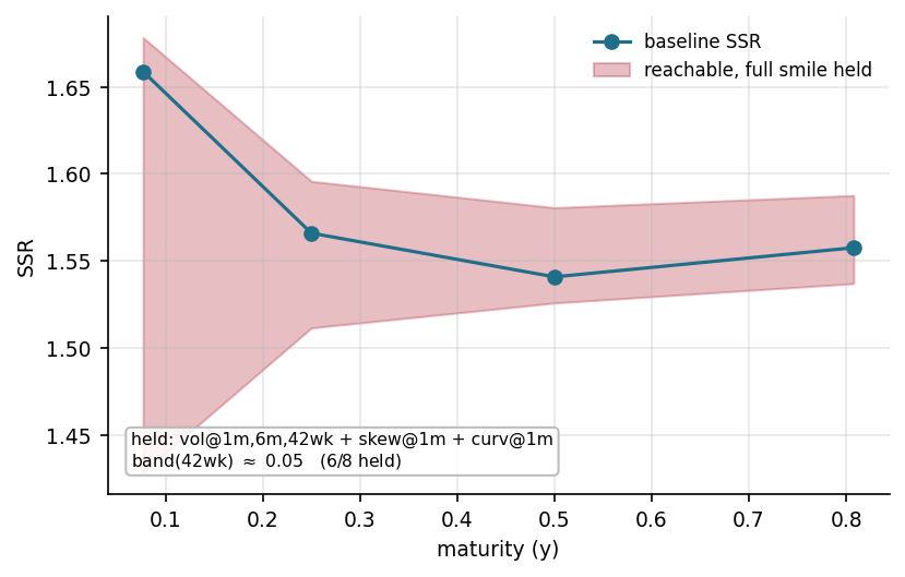
The dynamic degree of freedom is genuine but narrow. Hold the statics and ask how far the dynamics can still move. Along the steepest static-preserving
direction—the null space of the static Jacobian holding five smile observables (ATM vol at m, m and
weeks, skew and curvature at m), Newton-held to bp in the vols and in skew at every accepted
point—the -week SSR is freely movable only inside a band of width , , with six of eight walk points
holding (Figure 2). The freedom is thus non-zero—the family is genuinely stochastic-volatility, off the
local-volatility floor—and bounded: wider moves recruit the statics, which the full calibration supplies.
The direction that moves it is dominated by the slow factor, , and the projected gradient has
norm , so the reachable set is a thin sliver rather than a plateau. The moving direction is an
amplitude–persistence combination—the sensitivity map of Table 4 appearing in the null
space.
Figure 2. The statics/dynamics decoupling band at the shipped -- fit, computed on the construction
of Section 3. Moving along the steepest static-preserving direction, the SSR is confined to the
shaded band; its long end spans – at fixed statics, a width of . The band widens sharply at the
short end, where no observable is held.
5.2Data and calibration design
The real-data study calibrates one kernel per regime and reads it against two targets. Both underlyings
use the same design (Table 7); the one substantive difference is the forward-variance block,
risk-neutral on SPX and physical on NDX, which is the asymmetry the off-index study has to
overcome.
Table 7. Calibration design. The forward-variance block differs in measure and in observation
operator, both handled explicitly in Section 5.5. The SSR residual weighting differs for a measured
reason: on SPX the fitted target and the estimator behind the reported error band agree to at all
nine dates, whereas one NDX date carries a split between them (Appendix D), so off index the
residuals are weighted by their own measured reliability.
The design constants. Section 4 leaves the readout grids and objective weights symbolic because they are choices of this
study, not features of the model. Here they are. The kernel of Section 3 gives eight structural coefficients,
ordered , of which is pinned at zero, so the free dimension is . The tenor grid is with , so spanning one
week to three months. The forward-variance block runs from six to twelve on SPX, according to how
many VIX expiries survive the minimum-days filter, and is eight on NDX (, , , , , , , days). The objective
uses scaled by , so the two blocks carry comparable weight whatever their lengths, with a ridge toward
the stage anchor.
The counting condition is satisfied on both underlyings. On SPX the data-bearing residuals number to against seven free parameters; on NDX they
number , the realised strip being trusted at eight tenors for the reasons given in Section 5.5 and
Appendix D. The off-index fit is therefore over-determined by six coordinates. That is an absence of
underdetermination, not identification: it says the readouts outnumber the free parameters, not that they
pin them.
Fit quality is read against the target’s own precision. Each SSR target carries a joint heteroskedasticity- and autocorrelation-consistent standard error
(Appendix C), HAC’d across the regression slope and the skew denominator together since they are not
independent. We quote it as one number per year, the tenor-RMS of the relative standard error, and
report each fit against it. A residual smaller than that standard error is descriptive: it says the miss is
small relative to the target’s estimated sampling variability, not that model and target have been shown
equal, and not that the residual could not have been smaller. The band is a reporting benchmark:
nothing in the optimiser consults it, and it is not a stopping rule—the fits stop on xtol, as
Appendix E records. One row of Table 11 is an exception to the reading above: at NDX the fitted
target is the Huber-robust while the scale beside it is derived from the ordinary least-squares
estimator, so for that row the number is a precision scale from a different estimator, not that
target’s own standard error. With seven free parameters against five SSR tenors the kernel
can interpolate the point estimates outright, so the SSR block carries no positive residual
degrees of freedom and admits no in-sample specification test: agreement inside the band is
necessary and not sufficient. A test with positive degrees of freedom needs data withheld from
the fit, which Section 5.4 does. Both underlyings are inside the band at every date in the
panel.
All reported fits follow this protocol with no per-year tuning: one anchor, one schedule, one
resolution, for every date and both underlyings. The protocol, the numerical resolution and its
measured cost are in Appendix E; the realised-target construction and its four corrections are in
Appendix D.
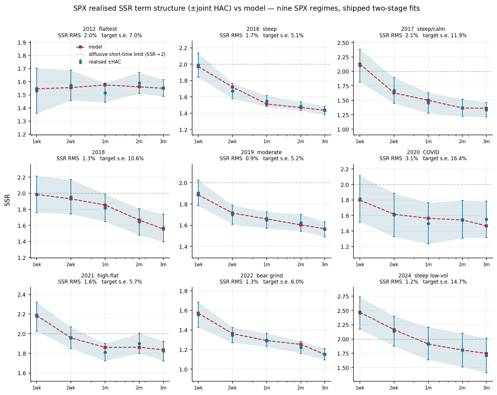
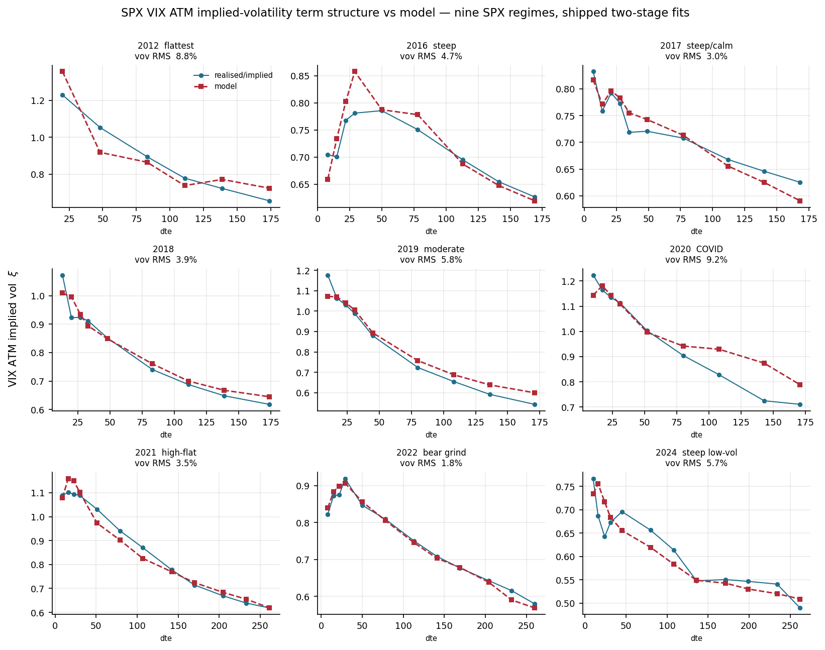
5.3SPX: cross-regime identification
Finding. Across nine SPX regimes—the flattest term structure (2012), the COVID shock (2020), the bear
grind (2022), the steepest low-vol surface (2024)—the kernel reproduces the realised SSR
term structure inside the year’s own sampling band at every date, and fits the VIX ATM
implied-volatility curve to – RMS. Each year is a single fixed calendar date, the first June trading
day.
Marginal compatibility. The statics layer and the kernel are mutually consistent before any dynamic target is imposed, and the
part of that consistency which is structural should be separated from the part which is measured.
Structural. The SANOS program is the joint linear program of Appendix A over all expiries at once,
whose calendar constraint imposes convex order on the fitted marginals across maturities to y.
Continuum convex order is a standing guarantee supplied by the marginal layer, which this paper takes as
a hypothesis rather than re-derives: the program enforces it as call inequalities on a strike
grid, so beyond the grid it rests on the smoothness of the mixture basis (Appendix A). The
propagated kernel satisfies positivity and normalisation at every state and parameter value, and
the martingale lock (23) at the numerical state the propagation carries, so the forward-start
return density has mass and forward equal to identically, not to within a tolerance. Measured.
Two things hold only up to an error that is reported. The local-variance level is matched to
leading order, its finite-step remainder (24) sitting in Table 8. And exact propagation of the
next spot marginal is the one admissibility condition the production chain does not inherit,
since the leverage overlay closes each step by collocation rather than by the exact Gaussian
identity (26). What the chain delivers is the finite-feature marginal compatibility of Definition 2, and
the condition it replaces is monitored rather than assumed: call-bp and IV-bp out to six
months, measured after the Gyöngy match of Section 3.3 and reported in Table 8. Those are
discrepancies at the quoted strikes, not a distance between laws, and no Wasserstein membership is
claimed.
What the empirical sections below test is the part the construction does not give for free—the
dynamics.
Dynamic fit. The calibration is a two-stage protocol rather than a single optimisation: a cold start, then a warm
continuation from it with the calendar derivative mollified at source, accepting the second stage only
where it lowers the data cost. It is deterministic, reproducible on any new date, and never worse than the
first stage by construction. Across the panel it improves both blocks—the SSR half of the objective by
and the forward-variance half by , for overall—and is accepted at four of nine dates (, , , ). It is the only
intervention we tested that improves the forward-variance fit without paying for it in the SSR
block.
The resulting SSR RMS averages and is inside the target’s joint-HAC standard error at all nine dates,
those bands running –; the VIX ATM RMS averages (Table 11, term structures Figures 3–4). Two
qualifications belong with those numbers. The acceptance test is in sample—one bit per date—and at two of the nine the margin is inside the objective’s own staircase noise, so the choice there is arbitrary, though
those are also the dates where it costs least either way. And the forward-variance instrument is biased: the
model’s VIX law sits low in forward while the VIX smile slopes up at in , so matching ATM volatility
identifies the vol-of-vol amplitude at a displaced point—a systematic, pooled over expiries, which is
the same order as the entire forward-variance residual. A moneyness-matched correction was
constructed and rejected: the displacement depends on , so lowering the amplitude and raising the
forward are substitutes, and the correction opened a flat direction rather than closing a bias
(Appendix D). The amplitude is therefore identified to within about ten percent, and we report it as
such.
External calibration of the level. A published estimate places the empirical SPX skew-stickiness ratio between and over –, at
maturities from one month outwards and on a -day rolling window [30]. Over that maturity range the
realised targets used here sit inside it at every tenor and every year (– from one to three months); the
fitted model leaves it once, at at one month; the one-week targets run higher, –, at a maturity the
published band does not cover.
That comparison anchors the level rather than bounding the variation. The skew-stickiness
ratio is an instantaneous ratio of covariations, so it is never observed, only estimated, and
the width of any reported interval mixes market variation with the variance of the estimator
behind it: the HAC standard errors of Appendix C run – of the target on the annual window
used here, hence roughly twice that on a sixty-day one, so a constant ratio of read through
such an estimator would print about at two standard errors—nearly the published interval
itself.
The more informative comparison is not the level but whether fitting the smile delivers the dynamics.
It does not. A two-factor Bergomi calibrated to the same smile does not reproduce the skew-stickiness
term structure, and the two-factor Quintic OU—a model built to target smile dynamics—reaches the
market range only once an SSR constraint is imposed alongside the smile [30]—consistent with the
inverse-problem argument of Section 1: skew-stickiness enters the observed range only when it is explicitly
constrained.
Stability across dates and optimizer basins. Three checks, reported in full in Appendix E. The joint objective is loosely identified: a cold start and
a warm continuation from a neighbouring fit can differ by up to points of SSR RMS, comparable to
the fit quality being reported. That freedom is bounded and measured: across four sensible
seeds the total data cost spans , the cold start best among them, while a seed taken from a
different tenor set lands one date worse—which is why the protocol fixes the seed rather
than searching over seeds. The parameters vary more than their fitted readouts do: any two
fits the protocol accepts reproduce the same SSR and skew term structures to within the
reported RMS, the residual freedom lying in the -directions those readouts leave soft (Table 12).
Section 6 draws the consequence. This is the decoupling of Section 3.3 seen from the calibration
side, and it is why the object carried downstream is the readout rather than . Repeating the
calibration at three static dates per year over – moves the fitted SSR term structure by a median
at one week and – from one to three months, inside the realised-SSR sampling band the fit is judged against. And the statics/dynamics decoupling holds regime-independently in the
variance: with the digital band given zero weight, so the kernel is fit to the dynamics alone, the
from-spot leveraged marginal still matches the SANOS marginals to survival RMS in calm,
high-vol and grind alike—the leverage carries the variance level whatever the dynamics do.
The digital band reads survival probabilities, which are integrals of the density and nearly
insensitive to an at-the-money slope, and the propagated skew does fall short of the target
marginal’s— of it at one week rising to at three months, on the same inversion at both sides. That
is a property of the overlay rather than of the fit, since a variance rescaling constrains no
third moment, and it does not enter the SSR readout, which normalises by the model’s own
skew.
Boundary. The two target blocks sit on different clocks—the SSR is an annual regression while the
marginal engine and the VIX curve are same-date cross-sections—and the static-date experiment above
measures the cost of that pairing.
Table 8. Architecture-level diagnostics on real SPX chains: what holds before and after the dynamic
fit, independently of the per-year fit errors of Table 11. The marginal row is measured after the
structural Gyöngy match, and is the finite-feature discrepancy of Definition 2 at the quoted strikes,
not a distance between laws. The leverage row is of (24), with both moments over the joint
factor-node/branch law, evaluated at the nodes the production step visits and weighted by the
production weights, so it is a probability-weighted summary rather than a maximum over tail nodes;
ranges are across the nine shipped fits.
Figure 3. Realised SSR term structure vs. model, one date per year, –. Markers, error bars and
shaded band: the realised skew-stickiness (a calendar-year regression) with its joint Newey–West
HAC SE, HAC’d across the regression slope and the skew denominator together since they are not
independent (Appendix C). Dashed: the model SSR at the fitted , from the two-stage protocol of
Section 5.3. Plain dashed line: the diffusive short-time limit , a continuous-time benchmark rather
than a bound on the finite-step statistic. The model sits inside the band at every tenor of
every date; each panel quotes that year’s RMS against its displayed precision scale, which on SPX
is the target’s joint-HAC standard error throughout.
Figure 4. VIX ATM implied volatility term structure vs. model, same dates. Markers: the
VIX-implied ATM volatility at every listed VIX-option maturity surviving the minimum-days
filter—six at , twelve by , so the fit is asked for more where the market provides more—a single-day
read carrying no sampling band. Dashed: model. On this underlying the readout and the target
are the same object, so no observation-operator correction is involved; the amplitude is however
identified only to within the instrument bias of Section 5.3.
5.4Held-out tenors: what the SSR block actually determines
Finding. The long end of the skew-stickiness curve is implied by the rest of the calibration; the short end
is fitted. Withholding the two interior tenors costs a median on the unseen points, below the target’s own
estimated standard error at eight of nine dates. Withholding the two end tenors costs a median , and the
damage is entirely at one week.
Design. Section 5.2 leaves the SSR block with no residual degrees of freedom; these create some.
Tenors are dropped from the objective by zeroing their entries in the residual weight vector, the survivors
renormalised so the retained block keeps its scale against the forward-variance block, and the model then
scored where it was not told the answer. Everything else—protocol, seed, box, ridge, forward-variance
targets—is the shipped configuration.
Table 9. Held-out SSR tenors, nine SPX dates. held RMS is over the two withheld tenors only; the
per-tenor columns are signed relative errors in percent. target s.e. is that year’s joint-HAC standard
error (Appendix C), an estimate of the target’s sampling variability. Excluding the interior held-out
RMS runs –.
interior: fit wk/m/m
ends: fit wk/m/m
Year
held RMS
wk m
held RMS
wk m
target s.e.
2012
2016
2017
2018
2019
2020
2021
2022
2024
median
inside s.e.
The two ends behave differently. Splitting the ends experiment by tenor, the three-month
error has median magnitude and no sign preference ( negative), while the one-week error
has median magnitude and is negative at seven of nine dates—a systematic undershoot,
not noise. Predicting the long end from the interior tenors and the forward-variance curve
works about as well as interpolating; predicting the short end does not. The model reaches the
realised one-week value when that value is in the objective, and does not get there on its
own.
Two independent results point the same way. The identifiability spectrum (Table 12) makes the slow
persistence the stiffest direction in the problem and the fast return correlation the softest; and the
diffusive short end is the first limitation listed in Section 6. What the held-out test adds is a magnitude
and a direction for a limitation that was previously asserted.
The interior failure is a shape failure, not a numerical one. With the two-week tenor withheld the
model places it at against a realised , between a well-fitted one-week () and one-month ()—a hump no
monotone decay would produce. It is not a numerical artefact of the ratio: (37) normalises by the model’s
own average skew and so diverges as that approaches zero, but the fit sits at , inside the – the panel spans
and well clear of the at which a parameter scan finds the readout diverging. That margin is recorded per
fit, which is what verifies the nondegeneracy hypothesis of Proposition 3 at the vectors the calibration
visits.
Boundary. Both designs withhold tenors within a date, not dates. The forward-variance block is fully
fitted throughout, the static surface is the same date’s, and the withheld and retained SSR targets come
from one panel of daily returns and are therefore correlated. This tests what determines the shape of the
SSR term structure; it is not out-of-time validation, and the annual target window of Section 5.2 is
untouched by it.
5.5NDX: portability, and what the off-index target actually measures
Finding. The model travels off SPX using no volatility-index data of the underlying’s own—the
targets are its own option strip and realised increments—though the observation-operator
correction those targets need is estimated on SPX and transported, which is the one imported
ingredient and is quantified below. It travels on both blocks: the SSR RMS is —inside the target’s
estimation band at all nine dates, and numerically close to SPX’s on a target built from NDX’s
own strip, though a residual inside one estimated standard error is a descriptive comparison
and not a test—and the eight-tenor realised variance-of-variance is fitted to against a target
carrying of its own roughness. The steep-decay shape gap that a nearest-expiry realised target
produces is substantially an observation-operator artefact rather than a limit of the two-timescale
decay.
The observation operator. The model’s forward-variance readout (43) prices an option expiring at on
a -day forward variance: the variance window is fixed and varies. On SPX the target is that same object.
Off index the target must be (51), the realised volatility of the -day variance-swap level, and the two are
not counterparts. The gap is quantifiable on SPX, the one underlying carrying both sides,
where the ratio is smooth and monotone in tenor, from at one week through unity near three
months to at six months, with nine to ten years of coverage at every tenor. Uncorrected
it is large enough to dominate: it makes the realised term structure appear to decay faster than a mean-reverting kernel can represent, and the demanded decay exponent falls from to
once it is applied—from outside the model’s reach to comfortably inside. The supporting
diagnostic is that SPX inherits the same apparent ceiling when fed realised targets, which
points at the target construction rather than at the off-index kernel without ruling the latter
out.
Four corrections, two checked on held-out tenors. The realised series needs a constant-maturity
construction (the nearest-expiry series rolls, and a realised volatility of a rolling series counts
each roll as a move); a physical validity bound (of observations exactly one lies outside the
range an index variance-swap level can occupy, and its single increment carried of that cell’s
annual variance); removal of increments spanning a bracketing-expiry change beyond three
months, where listed expiries are sparse enough that the switch is a genuine discontinuity; and
the observation-operator correction above. Two were checked on tenors withheld from the
fit. Fitting only the - and -day anchors and scoring the seven withheld tenors, each target
favours the run trained on it: the corrected-target run wins by a mean at nine of nine dates
when scored against the corrected series, and the raw-target run wins by a mean at seven of
nine when scored against the raw one. The correction is supported because the first margin
exceeds the second, not because either scoring is neutral. The held-out-tenor RMS is large in
absolute terms either way—– across the four combinations—so this ranks two targets rather than
validating a level. Fitting only – days, the churn removal predicts the held-out – day range
better—while dropping the same number of increments at random improves it by , so the gain is
attributable to those increments specifically and not to thinning a noisy series. Details, and two
statistical screens that were built and rejected on their own pre-specified diagnostics, are in
Appendix D.
What the remaining residual co-moves with. Measured as each year’s deviation from its own power
law—a shape the estimator has no reason to violate—the realised term structure carries RMS of
roughness against the model’s , a factor of five. Across the nine dates the fit residual and
that roughness correlate at with an intercept near : the cross-year variation in fit quality
moves with the target’s own smoothness. The daily coherence of the strip also degrades across
the sample—the first principal component of the eight-tenor increment panel explains of
variance in and by —which is itself a reason off-index calibration is harder than the index case.
Nothing here shows the off-index dynamics to be the same as SPX’s; what it shows is that the
instrument is measurably noisier, which is consistent with the residual gap without establishing
it.
What does not dissolve. One deficiency survives every correction, and it is visible on SPX rather than
NDX. Measuring each series against its own log-log shape, the model undershoots the forward-variance
readout at approximately six weeks by on SPX ( across the panel), against a traded VIX option price
with no correction, transport or estimator between model and observation. The same tenor
carries the largest residual on NDX (), amplified roughly fivefold by the noisier instrument;
the residual’s shape is common to the two underlyings (correlation ) while its amplitude is
not. We report this as a bounded limitation of the two-timescale decay rather than repair
it.
Boundary. The correction cannot be verified where it is applied, so Appendix D tests it on held-out
tenors instead. The SPX control bears on it in both directions: the residual oscillation is present on SPX
too, so it is not purely a transport artefact, but it is times larger off index. Separately, the off-index
marginal is modestly fat-tailed relative to the data (– the excess kurtosis), a discretisation
feature.
Figure 5. Off-SPX (NDX), both channels in one view, nine years. Filled circles: the realised-SSR
fit RMS. Shaded bars: that year’s displayed precision scale—the target’s joint Newey–West HAC
standard error, except at , whose target is the Huber-robust while the scale shown is OLS-derived
(marked in Table 11). Either way it is a scale to read the residual against, not a bound the residual
could not fall below. Open squares: the variance-of-variance fit RMS, a realised target carrying
no band of its own. Dashed line: that target’s measured roughness—its RMS deviation from its
own power law, . That is how far the target departs from its own smooth shape—roughness, not a
standard error and not a noise bound—so it carries none of the sampling interpretation the SSR
band does, and the line is the panel-average roughness rather than each date’s own. Every SSR
residual sits inside its band.
5.6What the calibrated kernel says about smile motion
Finding. The calibrated kernel places SPX on the sticky map in two independent coordinates: the smile’s
level rides with spot at the SSR, while its shape is very nearly frozen in moneyness.
Evidence. Taking the same exact- readout across the whole at-the-money neighbourhood rather than
at the level alone (Figure 6), the level responds as with running from at one week down to at three
months—far from sticky-moneyness (), between sticky-strike () and the local-volatility limit (),
and on the Doeff–Kamal backbone through the belly. The skew’s own response , normalised
by the rate at which a strike-pinned smile would swing it (twice the curvature), runs from
at one week to at three months: the shape is essentially frozen in moneyness, with a small
and realistic steepening on sell-offs that grows mildly with tenor. The one-month smile shifts
up nearly in parallel on a drop, unlike the flat sticky-moneyness or the tilted sticky-strike
responses.
Interpretation. The textbook equity picture comes out as a result rather than an assumption: the
fitted kernel holds the shape sticky and lets only the level ride, so the smile’s whole response to a spot
move collapses to the single number (39) folds into a delta.
Boundary. The frozen shape is a structural constraint as much as an empirical match: under the
translation invariance of Section 3 the conditional smile is a function of the volatility regime alone,
so shape responds to spot only through the leverage-induced regime shift. A deterministic,
spot-level-dependent shape lies outside the model’s reach.
Figure 6. Where the calibrated model sits on the sticky map (SPX, conditional-smile response to
a spot move, by moment). (a)Level: the SSR term structure, running at one week to at three
months, between the sticky-strike and local-volatility reference lines. (b)Shape: the one-month
smile’s response to a move, against the sticky-moneyness and sticky-strike references. The level
rides and the shape does not.
6Synthesis, limits, and conclusion
6.1What is identified
Fixing the marginals does not fix the dynamics. With five smile observables held to a few basis points, the
long-end skew-stickiness still moves across a band of width around the calibrated fit: the gap
European prices leave open is small enough to be a calibration target and large enough to
matter.
Fitting the two calibrated blocks narrows the kernel: across the nine-regime panel the SSR residual
RMS lies below the tenor-RMS estimated standard error at every date, and the forward-variance
residuals—whose target carries no sampling band—are reported separately (Section 5.3). But not
uniquely: distinct parameter vectors reproduce the same readouts along the soft directions Table 12
locates, median effective rank five of seven.
What the procedure identifies is therefore the tolerance set (28), a neighbourhood of the exact
class (27), with the block-specific tolerances of (28). The parameter vector is loose—two accepted fits can
differ by about a point of skew-stickiness RMS—while the readout it produces is stable under both
perturbations that matter, the static date it is calibrated on and the sample it is used out of. The readout
is what is carried downstream.
Read as a contract, that states what may and may not be claimed. Only outputs that are themselves
functionals of the selected readouts inherit the identification; other prices are model-implied. The
distinction bites precisely where it is tempting to ignore it: a forward-starting or path-dependent structure
is identified in this sense only to the extent that its value depends on the joint law through the first-order
spot–vol response and the forward-variance amplitude, and such prices can also depend on
joint tails and on higher-order features never sees. Two failures of identification then have
different remedies. Within the readout set are directions leaves soft, which Table 12 locates
and which sharper targets of the same kind would tighten. Outside it, statistics no chosen
readout sees are not weakly identified but unconstrained: the Zumbach effect and the broader
time-reversal asymmetry of volatility, any asymmetry in the vol-of-vol itself, and the joint tail
behaviour of spot and variance—[30] shows the question is live by testing the Zumbach effect
explicitly.
6.2What the two-timescale realization captures
Classical stochastic-local volatility also matches vanilla marginals and also produces smile dynamics; the
distinction is which quantities are independently imposed. There the residual spot–vol response falls to the
backbone, which is why calibrated backbones are documented to cluster [24]; here the overlay carries the
marginal level, leaving the innovation leverages and the two persistence loadings free to be identified
against an observed term structure.
Four features make the identification computable: the transition law is explicit, so prices, Greeks and
readouts are deterministic fixed-resolution evaluations rather than particle [14] or grid computations; the martingale property is enforced structurally, by the branch law, not by penalty; the fast/slow split gives
the spot–vol response a term structure with two interpretable timescales rather than a single decay; and
return–regime dependence runs through a shared branch index, coupling leverage and variance
dynamics inside the kernel rather than afterwards. Propagation stays in the finite-mixture class
throughout, which is what keeps the whole chain deterministic. Against frontier stochastic-local
volatility—multi-factor, rough, or neural—the edge is this combination, not dynamic control as
such.
6.3Limits revealed by the evidence
Four limitations survive the empirical study, each exposed by specific evidence and each pointing at a
different kind of extension (Table 10). The short end is the weak part of the fit, and the held-out test of
Section 5.4 measures how weak: withhold the one-week tenor and the model undershoots it by a median ,
at seven of nine dates, while the withheld three-month tenor is recovered to . The model skew-stickiness
also rises to the ceiling where SPX prints sub-month; the conditional smile shape is near-frozen in
moneyness, responding to spot only through the regime channel; in the off-index steep-decay years the
realised variance-of-variance falls from to days at a ratio against the kernel’s floor ; and
observationally equivalent parameter vectors populate the soft Jacobian directions. None is a numerical
defect.
Table 10. Limitations as a research map. The first two are consequences of the construction—the
translation invariance that makes the readouts exact closed forms is what freezes the conditional
shape—the third is a property of the two-factor family, and the fourth of the data available to
identify it.
One thing the evidence does not establish is a hedging edge. What is measured is a smile-roll residual
variance: the mean square of over each window—the part of the at-the-money move that
a one-parameter delta family leaves behind—with the strike slope and the return. It is
a proxy for hedging error, not a traded profit and loss: no vega weighting, no position, no
transaction cost. On that proxy the family is worth a great deal against no adjustment—
carries – the residual variance of the industry minimum-variance delta—and nothing against a
competent choice of . Out of sample on –, under the same train-only affine procedure, fitted
separately to each competitor, and a -row purge between train and test—the map is fitted on -day
forward outcomes, so without an embargo the last training rows would look into the first
test origins—the calibrated kernel’s own one-month readout, the corrected constant leg (the
input mapped to the training-sample target mean), an analytic smile-implied and a trailing
at-the-money regression are all within of the cross-strike Hull–White delta of [40] and of
each other. The kernel leg is served under a strict lag: each annual fit is calibrated to that
calendar year’s realised SSR, so on any date in year the forecaster uses the most recent fit
from a year strictly before , never the contemporaneous one. The minimum-variance delta
collapses to estimating one number, and one number is estimable many ways, so the model’s
dynamic content has nowhere to show up. Where it should show up instead is in quantities
the marginals cannot price at all—forward-start and path-dependent structures, whose very
definition needs the forward implied volatility the marginals leave open [18], and for which the
construction supplies deterministic finite-sum forward densities. That comparison is left to future
work.
Two limitations deserve a word. The value is the short-time limit of the skew-stickiness under a
diffusion, not a bound on the finite-step statistic: where the realised one-week value exceeds it—as it does
in the lowest-vol years, at –—the kernel follows it there. And the off-index residual combines the
two-factor decay floor with the physical measure in which that target must be quoted; the two cannot be
separated with the data available there.
6.4What would sharpen the identification
What would sharpen the identification is data, not a larger parameter count. The variance-index
smile—its skew and tails, not only the at-the-money level—reads the vol-of-vol shape under , and the
atomic variance-index law of Section 4.4 prices it across strikes with no new machinery; the forward-start
smile skew would supersede the realised proxy used here as the clean risk-neutral observable of spot–vol
leverage, but it needs cliquet quotes absent from listed feeds. The framework may also be adapted to
intraday surfaces, but jumps, seasonal liquidity, pinning and synchronized quote construction require a
separate model and dataset [31].
Two directions of extension follow from the architecture rather than from this instance of it:
the contribution is the architecture, not the two-factor kernel that occupies the framework
here.
Refining the topology. Enlarging shrinks both (27) and (28), so a new observable buys identification
rather than fit. It buys it only under two conditions, neither automatic. It must be expressible as a
functional of the discrete kernel—the readouts used here are closed forms because they are low-order
functionals of a Gaussian-mixture law propagated by the composition of Section 3.4, and a lagged cross-moment or a tail functional must be shown to be one. And it must carry identifying
power for the coordinates it is meant to pin, with the counting condition of Section 5.2 still
holding after whatever parameters it brings with it. The binding constraint is observables, not
flexibility.
Changing the occupant. The Gaussian-mixture kernel is a carrier, not a model. The two-timescale
latent-regime specialisation of Section 3.2 is one process placed inside it, chosen for span and tractability
rather than for economic commitment; the martingale lock, the leverage overlay that carries the
marginals, the recompression that holds the component budget flat, and the deterministic finite-sum
readouts are properties of the carrier. Any transition law expressible as—or approximable by—a Gaussian
mixture can be carried in the same machinery, which includes Markovian approximations of
rough kernels, further factors, and mixture components representing jumps. The cost is not
architectural but dimensional: the carried state and the recompression budget grow, and the
identification burden grows with the parameter count. The claims made in this paper are
about the architecture; the two-factor occupant is what the available observables can currently
support.
6.5Conclusion
European option prices identify marginals and leave the transition kernel open. This paper takes that
kernel as the unknown of an inverse calibration problem: the marginal layer is fixed independently by an
arbitrage-free engine, an explicit finite Gaussian-mixture family supplies the candidates, and a
representative of that family is calibrated to the specified skew-stickiness and forward-variance
readouts—up to readout equivalence—rather than fixed by a pre-selected process. What the
implementation delivers is weaker than the ideal admissible kernel it targets: martingality at the carried
numerical state before recompression, and marginal compatibility measured through finite-feature
discrepancies rather than imposed.
The evidence is that this works, and where it stops. The kernel fits nine SPX regimes to within the
target’s own sampling band; the skew-stickiness channel transfers to a second index on that
index’s own strip and realised increments, with the observation-operator correction those
targets need estimated on SPX and transported; and the residual—a shape gap in steep-decay
off-index years—is reproducible and bounded, and is consistent with a combination of the
two-timescale decay and the measure in which that target is quoted that the available data cannot
separate.
The broader implication is narrower than “dynamics can be calibrated from observed behaviour”,
which market models of implied volatility have done for two decades [32, 33, 34]. It is that the transition
kernel between fixed, convex-ordered marginals can be selected that way—in place of a transport
criterion, an entropic reference, or a prescribed stochastic backbone—and that the selection can be carried
out in a family explicit enough for the selecting quantities to be deterministic finite evaluations of its
own parameters, so that static no-arbitrage is a property of the construction rather than a
constraint the dynamics must be made to respect. The remaining limitations point toward
richer kernel families and fuller surface-level observations rather than a return to process-first
selection.
Acknowledgements. I would like to thank my fellow traders Yan Guo, Jun Liu, and Ge Yi for several conversations during the
preparation of this work.
AThe SANOS marginal-calibration LP
For completeness, Algorithm 1 states the SANOS static-layer calibration in this paper’s notation; the
original is [1]. It fits, per maturity, a weights-only Gaussian mixture whose call surface lands within
bid–ask and is arbitrage-free conditional on the continuum convex-order guarantee supplied externally by
the marginal layer—the program displayed below enforces the calendar inequalities on a strike
grid, not on the continuum—and free of butterfly and calendar arbitrage (positivity valid
density; forward constraint martingale; convex-order inequality calendar). The problem is
convex—a linear program for a piecewise-linear smoothing penalty , quadratic for a quadratic one.
Feasibility is a hypothesis on the quotes, not a property of the construction: when the bid–ask
bands admit a jointly arbitrage-free surface the fitted solution stays inside them, and when
they do not—mutually inconsistent quotes across strikes or maturities are not excluded a
priori—the program as written is infeasible and slack variables or soft quote penalties are required.
This is the admissible-marginal layer on which Theorem 1 and its convex-order precondition
rest.
Algorithm 1: SANOS marginal-calibration LP at maturity (this paper’s notation; after [1]).
Require: strikes with bid/ask , mids , weights ; forward ; fixed anchors in ; bandwidth ; previous-maturity fit Ensure: weights with , arbitrage-free on the enforced grid 1: Build the linear pricing map , the price of basis component at strike . 2: Solve the linear program over : 3: return ; the CDF is .
Two qualifications on the restatement. First, the convex-order condition appears above as a family of call
inequalities at grid strikes . As written that is numerical enforcement— exact at the grid points, and
beyond them only as far as the smoothness of the mixture basis carries it—rather than an exact finite
reduction of the continuum constraint. Second, this is a restatement in the present notation and not a
transcription: the authoritative formulation, and the precise sense in which its output is strictly
arbitrage-free, are [1], and where the two differ the original governs. Theorem 1 takes the convex
order of the delivered marginals as a hypothesis; this paper does not re-verify it on the fitted
surfaces.
BProofs of the approximation and stability results
Sections 2–4 use two mathematical facts, stated there as Propositions 2 and 3. This appendix proves
them, in the order in which each is used:
Both concern the construction of Section 3 as it is built: the
overlaid finite kernel, and the readout evaluated on it.
Notation. We keep the main text’s objects throughout: the lifted state with continuous, its law , and
the admissible kernels of Section 2.2, equation (5). In gross-return coordinates the martingale
constraint (19) is affine, , and a Gaussian log-return component is exactly a lognormal gross-return
component, so the two coordinate systems describe the same family.
Distances. On laws of the lifted state, is the -Wasserstein distance under the metric . On kernels we
use the integrated conditional distance
the source law being the lifted law the kernel is applied to.
Coefficient vectors carry the Euclidean norm on , and leverage functions the norm against the spot
marginal of the same .
B.1Martingality: the ideal statement and the implemented one
Two facts are used throughout and are separated because they condition on different -algebras. Both are
immediate from the coefficient map.
Proposition 4 (Ideal kernel, fibrewise) .For the intrinsic kernel with drift of (19), for every and every parameter value.
Proposition 5 (Implemented kernel, at its numerical state) .Let be generated by the component
index and the price abscissa the propagation carries. For the overlaid kernel with the lock (23),
and before the recompression projection, identically in the coefficients and in . The projection
that follows preserves mass and the unconditional forward but not this conditional identity, so no
martingale property is claimed for the reduced object.
Proof.Conditionally on a branch the increment is Gaussian, so . Averaging over the branches with
weights and inserting gives ; averaging instead over the joint quadrature with weights and
inserting gives the second statement.∎
Proposition 5 is the weaker of the two and is the one the production chain supports; every use of
“martingality is exact” in the main text refers to it.
B.2Standing hypotheses
All statements below are local, on a compact region of the implementation, and at a fixed numerical
pattern.
Assumption 1 (Nondegenerate region, fixed pattern) . (i) Coefficients. lies in a compact set with
; the log-variance clamp of Table 13bounds into , , uniformly in the node count. (ii) Local variance.
The regularised input satisfies and the spot-conditional variance ; is supplied by the marginal
engine and its convergence is external to this paper. (iii) Readout. Strikes are bounded away from
the wings; at-the-money Black vega is bounded below; the stationary average skew and the return
variance in (37) are bounded away from zero. (iv) Conditioning map. The spot-conditional variance
is stable in the source law: there is with for the adapted distance in use. This is assumed, not
derived: conditional expectations are not Lipschitz in weak or adapted topologies without further
structure, and we do not establish that structure here. (v) Source regularity and pattern. The
source kernel is Lipschitz in its state, with on the region—which is what lets one-step gaps be
propagated along the maturity grid. The branch and factor quadratures, the collocation rule and the
recompression partition are held fixed. Perturbations are in , in the local-variance input and in the source law—never in the pattern—so nothing below is a statement about refining the recompression,
and the paper makes no such claim (Section 2.3).
Part (i) is a hypothesis on the realised construction rather than a consequence of it. Two features make it
stable under refinement: the persistent factors are not discretised, so refining the remaining quadrature
refines an integral against a fixed Gaussian rather than enlarging the state space; and the
log-variance is clamped before exponentiation, so is bounded uniformly in the node count rather
than only at each fixed one. The resolution-agreement check of Section 5.2 is retained as a
diagnostic.
B.3Stability of the leverage pipeline
Proposition 6 (Local stability at a fixed numerical pattern) .Fix the numerical pattern of
Assumption 1(v). On the nondegenerate region, and given the conditioning hypothesis (iv), the
maps and are locally Lipschitz—the second in the integrated conditional Wasserstein distance (44),
with —and composing them along a finite maturity grid gives , where is the propagated-law gap
and the one-step kernel gap.
Proof.The first is the quotient rule with and , constant ; is bounded under the clamp. For
the second, each branch mean and variance is smooth in on the compact region and a Gaussian
mixture’s is bounded by the weighted sum of componentwise mean and standard-deviation gaps;
collect those bounds over the fixed node set. The recursion follows by inserting and using the
Lipschitz property of in its source.∎
Four limitations are part of the statement. The stability of the conditioning map is a hypothesis, not a
result—Assumption 1(iv)—so the chain of implications starts one step later than it appears to. It is local,
on a region assumed rather than derived. It holds at one fixed pattern: it says nothing about refining the
recompression partition, and in particular does not assert that the reduced chain converges to the unreduced one. And it concerns the overlaid kernel, not the full production pipeline—the recompression
projection of Section 3.4 is not a kernel and is not covered here; its effect is measured, not bounded.
Proposition 2 in the main text is this result applied to a convergent sequence of inputs at a fixed
pattern.
B.4Readout continuity
Theorem 7 (Readout regularity) .Under Assumption 1, each block of is locally Lipschitz in the
mixture state and in , and is therefore locally Lipschitz and piecewise in ; the pieces are the
segment boundaries of the calendar interpolation.
Proof. is a finite sum of normal CDFs with bounded below, and is globally Lipschitz; bare would
not suffice here, and the result uses the implementation’s explicit smooth mixture CDF. composes
the closed-form -step moments (40), a Gauss–Hermite sum of exponentials of affine functions under
the clamp, a square root away from zero, and the at-the-money Black inverse with vega bounded
below; the expiry variances satisfy for , so the node map is Lipschitz and no separate lower bound
on forward variance is assumed. is a finite sum of bounded factors over a return variance and a
stationary average skew, both bounded away from zero by Assumption 1(iii), with the trilinear
interpolant of (36) Lipschitz with the same constant as its data.∎
CThe realised-SSR sampling band (HAC)
The realised SSR markers and the shaded band in Figures 3 (SPX) and 5 (NDX) are a physical-measure
() estimate from a single year of daily end-of-day chains, so both the numerator and the denominator
carry sampling error that the band makes explicit. Comparing this target to the kernel’s
risk-neutral readout is motivated, at leading order, by the fact that the SSR is a ratio of one-step
covariations: quadratic covariation is measure-invariant—the / drift enters at and drops out
of the leading covariance—so the within-state comovement channel reads the same under
either measure to that order. Two limits on that argument should be kept in view. It does not extend to the between-state terms of the pooled annual regression, which can carry physical
drift and risk-premium variation that the risk-neutral kernel does not represent (Section 4
measures their size). And the band below quantifies sampling uncertainty of the empirical
pooled statistic; it is not evidence that the empirical and model functionals coincide. The
higher-moment vol-of-vol is not so protected (Section 5.2). At each tenor (; w to m) we regress
the daily ATM-forward implied-vol change on the daily log return with an intercept, and
divide the slope by the mean daily ATM skew at :
The ratio is Bergomi’s [22, 23], and as an
instantaneous ratio of covariations it carries no estimation window: the window is a choice,
not part of the definition. The calendar-year block used here follows from the calibration
design rather than from precedent—one kernel is fitted per regime, so one target is required
per regime. Published series may use much shorter windows, sixty days in [30] for instance,
which suits displaying the ratio as a time series; at that length the sampling band derived
below would exceed the fit errors of Section 5.3 several times over and so could not adjudicate
them.
Both pieces are estimated on the same days, so is a ratio of two jointly estimated quantities and its
standard error is not the combination of two separate ones. Treat as one M-estimator, with per-day
influence functions
where is the design matrix, and estimate their joint long-run covariance by a
Bartlett-kernel HAC, which guarantees a non-negative variance:
with the automatic lag –, so that .
The delta method applied to then gives
and the plotted strip is , one standard error per
tenor.
Two features of (48) are worth isolating, because the more familiar shortcut—a HAC slope error
combined with as though the two were independent—gets both wrong, and in opposite directions. The
daily ATM skew is strongly persistent within a year, so an iid standard error understates it: the
corresponding diagonal of inflates by a factor with median (range –), remarkably stable across tenors
and years. Against that, and are strongly positively correlated—HAC correlation at the median,
interquartile range to , positive in of the index-year-tenors—because a year with a steeper
mean skew is a year with a steeper vol–return slope. Both are negative quantities, so the
two entries of carry opposite signs and that common variation largely cancels in the ratio:
the cross term in (48) enters negatively, which no independent combination can represent.
This second effect is the larger, so the shortcut is not conservative in the way it looks—it
overstates , by a median across the eighteen index-years reported here, and by as much as .
The scalar band quoted in each panel title is this standard error as a single percentage—the
tenor-RMS of the relative error,
The band is a reporting benchmark, not part of the objective: the
kernel is fit to the point estimates in equal-percentage least squares (29), and nothing in the
optimiser consults the band—the fits stop on xtol. A fit whose SSR RMS falls below it sits,
on average, inside the -se strip; it is not the case that the residual cannot be smaller, since
the kernel carries more free parameters than the SSR block has tenors and can interpolate
the point estimates exactly. Nor is this a multivariate test: that would need the cross-tenor
covariance of together with positive residual degrees of freedom, and the second is unavailable
on this block whatever is done about the first. What the band fixes is a resolution below
which further reduction is not interpretable, so we stop there rather than chase sub-noise
structure. The strip widens at the short end, where the slope regression has the fewest effective
observations and the thinnest short-dated options. The forward-variance/VIX ATM implied volatility
readout (SPX, Figure 4) carries no band: it is a single-day risk-neutral () quote, not a sample
statistic.
A nonparametric check. Equation (48) is an asymptotic formula applied at , so we confirm it without the asymptotics. A
moving-block bootstrap resamples contiguous runs of trading days—block lengths , and , replicates—and
recomputes the entire statistic on each replicate: slope, skew mean and their ratio, with the blocks drawn
on common day indices across the five tenors so that the cross-tenor dependence the RMS band depends
on is preserved. Serial dependence is then carried by the blocks rather than modelled, and no
linearisation is involved. The resulting bands agree with (48) to a median ratio of (range –),
while both sit below the independent shortcut; the block length moves them by less than that
gap—two constructions this different agreeing is what licenses (48) at . No acceptance call
in Section 5 depends on the choice: every reported fit sits inside its band under all three
constructions.
DData construction and filters
Both realised targets are estimated on ORATS end-of-day chains. Neither is usable raw. This appendix
records every filter, the threshold it uses, and the evidence that it is inert where the data are already
clean; nothing here is tuned per year.
The realised skew-stickiness target. The realised SSR is a regression of daily ATM-vol changes on returns (Appendix C), so a single
corrupt print contaminates a whole year. Three filters precede it.
(i) Day spot. The day’s spot is the median stockPrice across the day’s smiles. ORATS records this
field per option row and it is unreliable—it varies across strikes and is corrupt by up to in –—so taking
any single row injects spurious one-day returns.
(ii) Positive fitted ATM skew. An index smile is always negative-skew, so a maturity whose fitted ATM
skew is positive on a given day is a corrupt short-dated quadratic fit through thin options, and that
maturity is dropped for that day.
(iii) Isolated short-end volatility spikes. Thin weeklies—pronounced on NDX—occasionally print an
absurd short-dated ATM vol (–, up to the one-month level, on calm days). These survive (ii), their skew
being negative. We drop a short maturity whose ATM vol exceeds the one-month: a genuine crash lifts
the whole curve and keeps the wkm ratio below , whereas the artifact is an isolated short-end
spike.
Rules (ii)–(iii) are inert on clean data. On liquid SPX they remove essentially nothing— bands and
fits are unchanged and the COVID crashes are retained—while on NDX // rule (iii) removes // corrupt
days, restoring the one-week SSR from – to – and its target standard error from – to –. NDX is the one
year where a large anti-leverage one-week print survives all three filters. Its effect is confined to the
shortest tenor and is large there: the ordinary least-squares returns at one week against under a
Huber-robust estimator, and the two agree to within at every other tenor. The OLS estimate also inverts
the term structure, placing the one-week value below the two-week one, which no index skew-stickiness
curve does. For that year, and only that year, the target is the Huber-robust , marked in
Table 11, where the scale shown beside it is OLS-derived rather than that target’s own standard
error.
Scheduled events are in scope by construction. Removing days adjacent to scheduled macro releases shifts the estimated SSR term structure by a median (max across –), almost entirely through —the
mean skew moves by under . The target therefore embeds scheduled-event risk, which is the
intended scope: the kernel is fit to the dynamics the market actually prices, not to a release-free
counterfactual.
The realised variance-of-variance target (NDX). NDX has no volatility-index options, and its variance-swap strip has only sparse monthly and
quarterly expiries past the front, so a fixed-tenor series built from the nearest expiry inherits a
spurious jump each time that expiry rolls. Each tenor is therefore built by the constant-maturity
interpolation (50). Three further corrections are needed before the series is a usable target, each arrived
at by measurement.
The estimator is the following. On trading day let be the model-free variance-swap volatilities at
every listed NDX expiry with days, each computed from that expiry’s out-of-the-money strip by the
standard log-contract replication. For a target tenor bracketed by , interpolate total variance linearly in
maturity and convert back to an annualised volatility,
with and the in the same units, so that the
day-count factor cancels and and carry the same annualisation, so is a volatility level in VIX units—not
a variance and not a total variance—and is the exact analogue of the quantity whose at-the-money option
the model prices in (43).
(i) A physical validity bound. Levels are restricted to in annualised volatility. This is not a percentile
but the range in which an index variance-swap level can exist at all. Of the NDX observations across
eleven tenors and ten years, exactly one lies outside it—a reading of , one basis point of volatility—and its
single increment carries of that tenor-year’s entire variance, driving the -day estimate to against
neighbours near . For scale the distribution is , median , , maximum . A bound of this kind cannot remove
signal: nothing trades at one basis point.
(ii) Adjacency. Days on which is not bracketed by two listed expiries are dropped rather than
extrapolated, and log changes are formed only between days that are adjacent in the trading calendar.
Letting a two-day change enter as if it were a one-day change is not innocuous at the thin tenors, where it
moves the estimate by up to (, days); at tenors with full coverage the two agree to within a few tenths of
a percent.
(iii) Bracket churn beyond three months. Constant-maturity interpolation removes the roll in the
target maturity but not in the bracketing pair: occasionally the near expiry rolls past or
a newly listed expiry slots in between, and the interpolation switches to a different pair of
smiles. Identifying the pair by absolute expiry date—not by days to expiry, which counts down
daily and would flag every day—such changes occur on of days but carry of the squared
variation. The structure across tenors is the reason the correction is applied only beyond three
months:
tenor
14d
21d
30d
45d
60d
90d
120d
180d
churn days (%)
59.2
58.6
52.2
33.4
19.1
5.7
8.7
7.5
churn / quiet
1.21
1.27
1.04
1.09
1.62
1.47
1.19
2.11
variance concentration
1.08
1.06
1.04
1.08
1.77
2.25
1.31
4.63
Where expiries are dense—weeklies at the front—a bracket switch is nearly seamless: frequent, but
ordinary. Where they are sparse, the pair spans a wide gap and the switch is a genuine discontinuity: rare,
but violent. Increments spanning a change are therefore dropped at days and beyond and
retained below; the -day tenor is recovered by this correction rather than excluded as an unlisted
gap-centre.
The target is then, with the retained days of the calendar year and ,
Three conventions are
choices and are recorded as such: log rather than percentage changes; demeaning rather than a
zero-mean second moment; and annualisation on trading days. The fitted tenors are , , , , , ,
and days. Seven days is excluded on coverage—it averages of trading days and is a single
day in three of the nine years—and / days on the absence of a bracketed volatility-index
quote against which to correct the observation operator. From days out coverage is at least
.
Two statistical screens were built and rejected, each by a diagnostic fixed before it ran. A
rolling-median filter on the log level was rejected because it screened hardest ( of points, cutting that
year’s -day estimate by ): its scale is the deviation from a lagging median, so a fast-moving year sets a
tight band precisely when the market moves. A round-trip test—flagging a large increment immediately
undone—was far more conservative () but bought almost nothing on an independent criterion it was not
designed for, namely that the term structure should decay with tenor: violations fell only
from to of , and got worse. Both, moreover, missed the one observation the physical bound
catches, the median filter because it re-centres on a corrupt neighbourhood and the round-trip
test because that observation sits at the start of its series and has no increment into it to
judge.
The observation operator, and correcting for it. The model side applies (43) at each fitted tenor, which is not the same functional as (51): one is the
implied volatility of an at-the-money option on the terminal law of at horizon , whose variance window is
fixed at thirty days; the other is the realised volatility of a time series of , whose window is itself. Both
are annualised volatilities of a volatility level, which is what makes the comparison meaningful,
but they are not counterparts, and the gap between them widens with because the realised
object grows smoother as its own tenor lengthens while the readout stays pinned at thirty
days.
SPX is the one underlying carrying both sides, so the gap is measurable rather than assumed. Pricing
the VIX-implied at-the-money volatility against a realised variance-of-variance built from SPX’s own
strip by the identical construction, the ratio is smooth and monotone in tenor— at seven days, at thirty,
crossing unity near three months, at six—over nine to ten years of coverage at every tenor. Two effects of
opposite sign are netted in it and this measurement does not separate them: a volatility-risk premium,
which lifts the side, and the fact that vol-index options are written on futures whose volatility is damped
by mean reversion relative to the spot the realised side measures, which lowers it. Neither is the largest
term: the functional mismatch above is, and it is pure construction rather than measure.
Applied per year and per tenor, the correction moves the demanded decay exponent from to
.
What can be checked, since the correction cannot be verified where it is applied, is whether it improves
prediction on tenors the fit never saw: fitted at the - and -day anchors alone, the corrected-target run
beats the raw-target run on the seven held-out tenors by a mean at nine of nine dates under
corrected scoring, against a win at seven of nine for the raw-target run under raw scoring; absolute held-out RMS runs –. Each scoring favours its own training object, so what supports
the correction is the gap between those margins. The churn correction was checked the same
way and against a control: fitted at – days alone, it improves held-out – day prediction by ,
while dropping the same number of increments chosen at random improves it by over forty
draws. The gain is attributable to those increments specifically and not to thinning a noisy
series.
What the cleaning does to the conclusion. Much of the apparent steep-decay shape gap co-moves with the observation operator rather than with
the kernel, and the supporting diagnostic is that SPX inherits the same apparent ceiling when fed realised
targets. That is consistent with target construction contributing materially; it does not exclude kernel
misspecification. What survives is stated in Section 5.5.
ECalibration protocol and robustness
One protocol is used for every reported fit. This appendix states it, quantifies the multi-basin freedom
that makes an acceptance rule necessary, and reports the robustness experiments summarised in
Section 5.3.
Objective. The objective is (34) at the design constants of Section 5.2, with no per-year tuning anywhere and
one documented difference between the two underlyings: the skew-stickiness weights . On SPX they are
unity, so the five tenors enter equally. On NDX they are the inverse of each tenor’s own measured
relative HAC standard error, normalised to . That normalisation is what keeps the choice
from being a second lever: the SSR block’s expected squared magnitude is unchanged, so the
SSR-versus-forward-variance balance is untouched and the weighting only redistributes within the
block. The reason it is applied off index is that the off-index targets are far more unevenly
determined—at NDX the one-week standard error is of the target against at three months,
so equal weighting spends the fit on the least-determined cell. Realised weights run from
to across the nine dates, their spread widest where the short-tenor errors are. One caveat
travels with the choice: the recorded standard error is the ordinary least-squares estimator’s,
so at NDX —the single date whose fitted target is the Huber-robust —the weight and the
target come from different estimators. The number reported beside that target is therefore an
OLS-derived precision scale, not an uncertainty measure for the robust estimate; we have not
computed a compatible robust one, and it should not be read as that date’s target standard
error.
At the five tenors wk–m the SSR target is an ordinary least-squares over a calendar-year window
after the filters of Appendix D; the one exception, NDX , is discussed there. The ridge is taken toward the
current stage’s anchor —the fixed uniform start in the cold stage, the cold stage’s own optimum in the
warm one—so the warm refinement is regularised toward where it begins rather than toward a fixed point
of the parameter box.
Numerical resolution: one setting, and no ladder. The propagation does not discretise the volatility factors into abscissas the kernel walks: they are
carried continuously and integrated, so refining the readout is an ordinary quadrature refinement of a fixed
Gaussian rather than an enlargement of the state space. There is consequently no node ladder, and no
node-count convergence question distinct from the quadrature limit.
Every fit reported here therefore runs at a single fixed resolution, and the readout’s sensitivity to it is
measured rather than assumed. Holding the fitted and refining every quadrature the readout touches
moves the forward-variance reading by at most , monotonically decreasing and growing mildly with tenor;
the SSR block does not pass through that path and does not move. Splitting the refinement shows
roughly two-thirds of it is quadrature and one-third the recompression budget, the two being
additive to within percentage points. Several quadratures—in particular the stationary bivariate
grid—leave the readout bit-identical at any setting, since the closed-form step law does not consult
them.
The leverage overlay’s finite-step remainder. The overlay matches the continuous relation (21) to leading order, and (24) names what is left over.
Evaluated by leverage_remainder.py at the nodes the production step visits and with the production
weights, has a probability-weighted RMS of – across the nine shipped fits and a weighted median of –; the
th weighted percentile runs –, worst at .
Because is a relative variance error the corresponding volatility error is about half of it: roughly bp of
implied volatility at RMS on a surface at the best date and about bp at the worst, against the
IV-bp marginal discrepancy the overlay exists to close (Table 8). At most dates the remainder
is well inside that residual; at and —the two steep-leverage years—it is of the same order,
and at the worst date it exceeds it. We report it rather than repair it: correcting it would
require an exact scalar solve for at every price abscissa and a full recalibration. That is the
honest statement of the trade—the remainder is a known, measured approximation of the same
magnitude as the marginal discrepancy at the two steepest dates, not one demonstrably below
it.
The resolution is chosen on cost. Each refinement step multiplies the readout cost by roughly six, so a
fully refined reading is about times the production one: the -minute panel below would take over three
days. Against a readout bias on one of the two blocks, that is not a trade worth making for
a model intended to be recalibrated daily, and the bias is reported instead. Its direction is
known and favourable: the production reading overstates the forward-variance level slightly
and more so at longer tenors, so the reported forward-variance residuals are, if anything,
conservative—and the model’s vol-of-vol term structure is marginally steeper than the reported figures
imply.
Cost, per year. Every fit reported here was produced on one Apple-silicon GPU (mps) at the single fixed resolution
above, and the wall time is recorded in each fit record rather than estimated. Stage 1 (cold) runs – s per date and stage 2 (warm) – s, stage 1; the protocol costs both at every date before
the acceptance rule can compare them, minutes across the nine SPX dates. Off index the
eight-tenor NDX panel is a single cold stage, minutes in total. Fits take – objective and – Jacobian
evaluations, so a single-date recalibration is a few minutes—the operating point the design
targets.
Determinism. The accelerated backend is bit-deterministic on device: repeated evaluation of the same reproduces
the residual and the Jacobian exactly. It matters most for the Jacobian—forward tangents pass through
segment-boundary comparisons, where a boundary flip changes the derivative structure outright rather
than perturbing its value—and it costs about on a whole fit, leaving the accelerated path roughly thirteen
times faster than the reference loop it replaces.
Table 11. Fit quality across regimes and underlyings, RMS in percent. Every SSR entry lies
below its displayed precision scale. Except for the daggered row, that scale is the target’s
joint-HAC standard error (Appendix C); the daggered scale is OLS-derived. This bounds what may
be claimed about the fit, and is not a specification test (§5.2). is the number of forward-variance
constraints—on SPX whatever VIX expiries were listed, on NDX the eight tenors of the corrected
realised strip. The SPX two-stage protocol accepted its second stage at 2012, 2016, 2017 and 2018.
The NDX forward-variance column should be read against the target’s own roughness (Section 5.5)
rather than against zero: roughness co-moves strongly with residual size, which is consistent with
target construction contributing materially but does not exclude kernel misspecification; the SPX
column is subject to the instrument bias of Section 5.3.
SPX (forward variance from VIX)
NDX (realised strip, -weighted SSR)
Date
regime
SSR
s.e.
vov
SSR
s.e.
vov
2012
flattest
6
8
2016
steep
9
8
2017
steep/calm
10
8
2018
—
9
8
2019
moderate
9
8
2020
COVID
9
8
2021
melt-up
12
8
2022
bear grind
12
8
2024
low-vol
12
8
mean
Multi-basin freedom, measured. The joint objective admits several basins and a poor seed can settle in one: seeding an off-index panel
from a fit made against a different tenor set lands one date worse on its own objective and the panel
worse. But the cold start is not one of the poor seeds, and the freedom among sensible ones is
small. Holding the objective and the targets fixed and varying only the seed—cold, a warm
continuation from the fit’s own solution, and warm continuations from two independently
converged fits—the total data cost spans –, a range of , with the cold start the best of the
four; taking the per-date minimum across all four, which is in-sample selection and reported
only as a bound, buys —an order of magnitude smaller than the fit quality. What is loosely
identified remains the parameter vector rather than the priced dynamics: any two fits the protocol
accepts reproduce the same SSR and forward-variance term structures to within the reported
RMS.
The identifiability spectrum, measured. Table 12 carries it. At each fitted the elasticity-scaled readout Jacobian is formed over the seven free
coordinates at the shipped configuration, with , and its singular values recorded. It is the readout map
that is differentiated, not the residual vector of (33): the objective weights and the ridge are excluded, so
the spectrum describes what the observables determine rather than what the optimiser saw. Two readings
matter. The conditioning is not uniform across regimes: the ratio runs from to , and the
number of directions above of the leading one—an effective rank at that tolerance—from two
to six, median five out of seven. So the readout vector determines most but not all of the
parameter vector, and how much depends on the year. The second reading is which coordinates sit
in what is left over. Averaging the softest singular vector’s loadings across the nine dates
orders the parameters cleanly: carries of it and carries . The fast return correlation is the
softest direction in the problem and the slow persistence is the stiffest—which is the reverse of
what the parameters’ roles would suggest, and is the reason a fitted should not be read as a
measurement.
Table 12. Elasticity-scaled readout-Jacobian spectrum at the nine shipped SPX fits, seven free
coordinates—the readout map differentiated, objective weights and ridge excluded—generated from
jacobian_7free_ALL.json by emit_jacobian_table.py. stage is which stage of the two-stage
protocol that date’s shipped fit came from. The lower block averages the softest singular vector’s
loadings over the nine dates, sorted.
Year
stage
rank
2012
warm
11
2016
warm
14
2017
warm
15
2018
warm
14
2019
cold
14
2020
cold
14
2021
cold
17
2022
cold
17
2024
cold
17
median
Replication manifest. Table 13 lists the numerical constants the production path reads. It is not transcribed: it is emitted by
emit_manifest.py directly from the objects the calibration constructs, or parsed from the fitter’s own
source, so it cannot drift from the engine. Values shown are the on-index defaults; off-index
overrides are recorded per record. The same script writes manifest.json, carrying the box,
per-date wall time, objective and Jacobian evaluation counts, the device, and for every record
on both underlyings a truncated (-hex-character) sha-256 fingerprint and a reproduction
check.
Each record states its own leverage-ladder configuration, so stage 2’s source mollification (LAMH ,
PILLARAWARE ) is legible from the artifact and not only from the protocol. That claim is checked
rather than trusted: each record’s own is re-evaluated under both candidate ladders and compared
elementwise against that record’s own stored readout. On the device the fits were produced on, every one
of the nine reproduces bit-exactly under the ladder it declares, and misses by – under the other—so the
declaration and the numbers agree, by two independent routes. Off the device the fits were produced on,
the same exercise reproduces each record’s declared ladder but not its numbers exactly. On the one
alternative device tested (cpu against mps, both float), the artifact records two quantities across the
nine dates: the SSR-RMS gap runs – percentage points, and the mean relative elementwise
deviation of the readout –. Those are observations on one device pair, not a bound for arbitrary
hardware.
Code and data availability. The replication bundle is built by make_release.py, which walks the import graph from
five entry points—the fitter refit.py, the two table generators, the leverage diagnostic and
the smile-roll harness—and copies the resulting closure. It is modules, not the six of the
production path alone: those import path, band, smile and calibration helpers that a reader needs
and the paper does not name. Two of the five need the option chains and so cannot be run
from the bundle alone, refit.py and the smile-roll harness; the other three were checked by
extracting the archive outside the source tree and running them there. Alongside the code the
bundle carries the eighteen SPX and NDX fit records, the artifacts the tables are generated
from (manifest.json, the readout-Jacobian spectrum, the leverage-remainder summaries), an
environment lock, a README, and SHA256SUMS giving a full sha-256 for every file shipped. It
is not a copy of the working directory: superseded scripts, backup files, build output and
the archived long-form appendix are absent by construction. Available from the authors on
request. The option chains are licensed ORATS data and cannot be redistributed; Appendix D
gives the filters and target constructions in enough detail to rebuild them from an equivalent
source.
Table 13. The principal production configuration—the constants a reader must set to reproduce
the fits, not an exhaustive list of every literal in the path (the skew-difference step , the eight
Newton iterations of the at-the-money inversion and the -step VIX bisection are fixed in the code
and not exposed)—emitted by emit_manifest.py. The quadrature counts, the box, the clamps
and the optimiser settings are read from the objects the calibration constructs or parsed from the
fitter’s own source, so none of them is transcribed.
, the shipped --fit. Reaching the long end needs a snapshot grid at weeks rather than the five fitted tenors; the
leverage ladder is the shipped -week one, so weeks is the longest tenor the production configuration supports and the band is
quoted there rather than at one year. ↩
[2]Dupire, B. (1994). Pricing with a smile. Risk, 7(1), 18–20.
[3]Breeden, D. T., Litzenberger, R. H. (1978). Prices of state-contingent claims implicit in option prices. Journal of Business, 51(4), 621–651.
[4]Derman, E., Kani, I. (1994). Riding on a smile. Risk, 7(2), 32–39.
[5]Rubinstein, M. (1994). Implied binomial trees. Journal of Finance, 49(3), 771–818.
[6]Gyöngy, I. (1986). Mimicking the one-dimensional marginal distributions of processes having an Itô differential. Probability Theory and Related Fields, 71(4), 501–516.
[7]Jex, M., Henderson, R., Wang, D. (1999). Pricing exotics under the smile. Risk, 12(11), 72–75.
[8]Lipton, A. (2002). The vol smile problem. Risk, 15(2), 61–65.
[9]Heston, S.L. (1993). A closed-form solution for options with stochastic volatility with applications to bond and currency options. Review of Financial Studies, 6(2), 327–343.
[11]Gatheral, J. (2006). The Volatility Surface: A Practitioner’s Guide. Wiley.
[12]Brigo, D., Mercurio, F. (2002). Lognormal-mixture dynamics and calibration to market volatility smiles. International Journal of Theoretical and Applied Finance, 5(4), 427–446.
[13]Ren, Y., Madan, D., Qian, M.Q. (2007). Calibrating and pricing with embedded local volatility models. Risk, 20(9), 138–143.
[14]Guyon, J., Henry-Labordère, P. (2012). Being particular about calibration. Risk, 25(1), 92–97.
[15]Guo, I., Loeper, G., Wang, S. (2022). Calibration of local-stochastic volatility models by optimal transport. Mathematical Finance, 32(1), 46–77. (First version: arXiv:1906.06478, 2019.)
[16]Cuchiero, C., Khosrawi, W., Teichmann, J. (2020). A generative adversarial network approach to calibration of local stochastic volatility models. Risks, 8(4), 101.
[17]Jourdain, B., Zhou, A. (2020). Existence of a calibrated regime switching local volatility model. Mathematical Finance, 30(2), 501–546. (arXiv:1607.00077.)
[18]Glasserman, P., Wu, Q. (2011). Forward and future implied volatility. International Journal of Theoretical and Applied Finance, 14(3), 407–432.
[19]Strassen, V. (1965). The existence of probability measures with given marginals. Annals of Mathematical Statistics, 36(2), 423–439.
[20]Beiglböck, M., Henry-Labordère, P., Penkner, F. (2013). Model-independent bounds for option prices—a mass transport approach. Finance and Stochastics, 17(3), 477–501.
[21]Beiglböck, M., Jourdain, B., Margheriti, W., Pammer, G. (2022). Approximation of martingale couplings on the line in the adapted weak topology. Probability Theory and Related Fields, 183, 359–413.
[22]Bergomi, L. (2009). Smile dynamics IV. Risk, 22(12), 94–100.
[23]Bergomi, L. (2016). Stochastic Volatility Modeling. Chapman & Hall/CRC.
[24]Bergomi, L. (2017). Local-stochastic volatility: Models and non-models. Risk, August 2017, 78–83.
[25]Gatheral, J., Jaisson, T., Rosenbaum, M. (2018). Volatility is rough. Quantitative Finance, 18(6), 933–949.
[26]Bayer, C., Friz, P., Gatheral, J. (2016). Pricing under rough volatility. Quantitative Finance, 16(6), 887–904.
[27]Friz, P. K., Gatheral, J. (2024). Computing the SSR. arXiv preprint arXiv:2406.16131.
[28]Fukasawa, M. (2026). On the skew stickiness ratio. arXiv preprint arXiv:2602.05241.
[29]Bourgey, F., De Marco, S., Delemotte, J. (2024). Smile dynamics and rough volatility. SSRN preprint 4911186.
[30]Abi Jaber, E., Li, S. (2025). Capturing Smile Dynamics with the Quintic Volatility Model: SPX, Skew-Stickiness Ratio and VIX. arXiv preprint arXiv:2503.14158v2 (revised 21 April 2026).
[31]Bandi, F. M., Fusari, N., Gazzani, G., Renò, R. (2026). Ultra-short-term volatility surfaces. arXiv preprint arXiv:2603.29430.
[32]Schönbucher, P. J. (1999). A market model for stochastic implied volatility. Philosophical Transactions of the Royal Society A 357(1758), 2071–2092.
[33]Cont, R. and da Fonseca, J. (2002). Dynamics of implied volatility surfaces. Quantitative Finance 2(1), 45–60.
[34]Cohen, S. N., Reisinger, C. and Wang, S. (2023). Arbitrage-free neural-SDE market models. Applied Mathematical Finance, 30(1), 1–46. (arXiv:2105.11053.)
[35]Guyon, J. (2025). Dispersion-constrained martingale Schrödinger bridges: Joint entropic calibration of stochastic volatility models to S&P 500 and VIX smiles. SIAM Journal on Financial Mathematics, 16(3), 834–874. doi:10.1137/22M1511242. (Earlier: SSRN preprint 4165057.)
[36]Guo, I., Loeper, G., Oblój, J., Wang, S. (2022). Joint modeling and calibration of SPX and VIX by optimal transport. SIAM Journal on Financial Mathematics, 13(1), 1–31. doi:10.1137/20M1375905. (arXiv:2004.02198.)
[37]Guyon, J. (2024). Dispersion-constrained martingale Schrödinger problems and the exact joint S&P 500/VIX smile calibration puzzle. Finance and Stochastics, 28(1), 27–79.
[39]Doeff, E., Kamal, M. (2012). Consistent and realistic dynamics of the implied volatility surface under local volatility models. SSRN preprint 2207171.
[40]Hull, J., White, A. (2017). Optimal delta hedging for options. Journal of Banking and Finance, 82, 180–190.
[41]Andreasen, J., Huge, B. (2011). Volatility interpolation. Risk, 24(3), 76–79.
[42]Conze, A., Henry-Labordère, P. (2021). Bass construction with multi-marginals: Lightspeed computation in a new local volatility model. SSRN preprint 3853085. (Condensed version: A new fast local volatility model, Risk, April 2022.)
[43]Backhoff-Veraguas, J., Beiglböck, M., Huesmann, M., Källblad, S. (2020). Martingale Benamou–Brenier: a probabilistic perspective. Annals of Probability, 48(5), 2258–2289.
[44]Qin, H., Che, C., Yang, R., Feng, L. (2024). Robust and fast Bass local volatility. arXiv preprint arXiv:2411.04321.
[45]Hunt, P., Kennedy, J., Pelsser, A. (2000). Markov-functional interest rate models. Finance and Stochastics, 4(4), 391–408.
[46]van den Berg, T. (2026). Mixture-preserving, arbitrage-free interpolation for volatility-surface models. arXiv preprint arXiv:2606.12717v2 (15 June 2026).
How to cite
Shaosai Huang (2026). SANOS-Evolve: A Discrete Stochastic-Local-Volatility Model for European-Option Smile Dynamics. Working paper, version 3, July 2026. Kspectra Research. SSRN 7151258 (doi:10.2139/ssrn.7151258). https://kspectra.ai/papers/sanos-evolve/
@misc{huang2026sanos,
  author = {Huang, Shaosai},
  title  = {{SANOS-Evolve: A Discrete Stochastic-Local-Volatility Model for European-Option Smile Dynamics}},
  year   = {2026},
  month  = jul,
  note   = {Working paper, version 3, July 2026},
  doi    = {10.2139/ssrn.7151258},
  url    = {https://kspectra.ai/papers/sanos-evolve/}
}