The Right Wing of the SABR Smile with an Absorbing Boundary: Resolution of Conjectures of Henry-Labordère
Zeyu Cao1 and Shaosai Huang2
∗ Working paper. Comments welcome.
1 Independent Researcher, Long Island City, USA
2 Kspectra Research Inc., Toronto, Canada
Abstract
We determine the leading logarithmic asymptotics of the fixed-maturity right tail of the SABR model with and absorption at zero, for every correlation . If is the probability that the terminal forward is at least , then
For this is the rate predicted by the unrestricted hyperbolic geometry. For it is strictly larger: along the volatility excursion that produces the tail, survival forces the noise orthogonal to volatility to stay above a moving square-root barrier, at an additional cost of the same order . Consequently the Black–Scholes implied volatility tends to : Henry-Labordère’s conjectured wing limit holds for and fails for every . For his second conjecture, whose unrestricted-distance Gaussian estimate does not hold for , we also identify the correct replacement for this model: at the level of tail probabilities, the rate is given by the squared intrinsic Riemannian distance, within the survival domain, from the initial state to the terminal target set. The proofs are direct, combining a stopped Lamperti transform, a conditional time change, Gaussian moving-barrier bounds and change-of-measure constructions, and use no heat-kernel estimates.Contents
Absorption can alter a fixed-time logarithmic tail asymptotic even when the absorbing boundary is
disjoint from the terminal target set. We establish this phenomenon for the SABR diffusion absorbed
at zero: the volatility excursion that produces a large terminal value can simultaneously drive the
forward toward the boundary, so paths contributing to the right tail incur an additional
Brownian boundary-crossing cost. The main theorem concerns the terminal right tail of the
absorbed diffusion; the implied-volatility wing then follows from a model-free transfer
principle.
1.1The Problem and Henry-Labordère’s Conjectures
The SABR model of Hagan, Kumar, Lesniewski and Woodward [HKLW02] is a widely used
stochastic-volatility parametrization of implied-volatility smiles in interest-rate markets and beyond:
with , , , and . Precisely, we work on a complete filtered probability space satisfying the usual
conditions and carrying independent standard Brownian motions . We set and
On the open state
space , is the pathwise-unique strong solution of the first equation in (1.1) up to the absorption time
and we take the continuous absorbed extension for . This boundary condition is part of the model:
it selects the absorbing continuation among the possible post-hitting extensions of the
CEV equation. Throughout, is a fixed maturity, is the log-moneyness, and denotes
the Black–Scholes implied volatility of the undiscounted call with strike and maturity
.
At fixed maturity, the extreme right wing probes joint rare excursions of volatility and the
forward. The unrestricted hyperbolic geometry of the model suggests a correlation-independent
leading coefficient, whereas the right-tail event for the absorbed process requires survival in . The
question is whether this survival constraint is negligible on the leading scale.
In Chapter 10 of his monograph [Hen08], Henry-Labordère writes the generator of a
stochastic-volatility model as a Schrödinger-type operator on a Riemannian manifold: a
Laplace–Beltrami part determined by the diffusion matrix, a connection one-form, and a scalar
potential . Assuming a Gaussian bound of Li–Yau–Davies type [LY86; Dav89] for the
associated heat kernel (his (10.21)), he obtains a wing formula, his (10.22), in which the
extreme strikes are governed by the geodesic distance, in the unrestricted metric, from the
initial point to the terminal fibre . For SABR this metric is hyperbolic, and the resulting
limit is . Let denote the volatility coordinate of the point of the fibre nearest to the
initial point, that is, the saddle point of the fibre integral. For SABR with , the scalar
potential along this saddle has the large-strike limit given in [Hen08, p. 306]:
The potential
is therefore bounded along the far-right saddle. On the strength of this boundedness,
Henry-Labordère poses two conjectures, which we restate in our notation, keeping his
numbering.1
Conjecture 1 ([Hen08, p. 306]).For SABR with , as , for every .
The second conjecture concerns the Gaussian estimate itself.
Conjecture 2 ([Hen08, p. 306]).If the potential is bounded, the Gaussian wing estimate
(10.22) of [Hen08] is valid.
Conjecture 1 is the proposed right-wing limit; Conjecture 2 would justify the
unrestricted-distance Gaussian estimate from the boundedness of the potential at the saddle point.
As the book notes, Conjecture 1 was proved for by Benaim, Friz and Lee [BFL08]. To our
knowledge, the fixed-maturity correlated case , has remained open (see Section 1.4). The
difficulty is the gap between evaluating a coefficient at the unrestricted saddle point and
controlling the Dirichlet semigroup of the diffusion killed at the boundary of its state
space.
1.2Main Results
We measure the right tail by the probability that the terminal forward ends at or above a large
strike, and compare its decay with two quadratic rates:
For the rate exceeds , and our main result
shows which of the two governs the tail.
Theorem 1.1 (Logarithmic Right-Tail Asymptotics for Absorbed SABR).For every ,
Through a model-free transfer from tail probabilities to call prices (Lemma 2.3), the decay rate
determines the right wing of the implied-volatility smile.
Corollary 1.2 (Right-Wing Implied-Volatility Limit).For every ,
Comparing this limit with Henry-Labordère’s prediction settles Conjecture 1.
Corollary 1.3 (Resolution of Conjecture 1).For every , the conjecture holds for and fails for
every . The wing limit
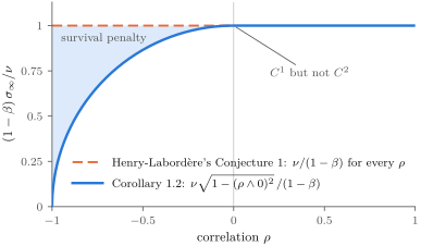
as a function of , is but not at : its second derivative from the left is and
from the right is . It does not depend on , or , and depends on only through the factor
.
Both corollaries follow from Theorem 1.1 and the integrability alone. Figure 1 shows the limit as
a function of , together with the value predicted by Conjecture 1.
Figure 1. The right-wing limit of Corollary 1.2, normalized by , against the correlation .
Henry-Labordère’s Conjecture 1 predicts the value for every . It holds for ; for survival lowers the
limit to (shaded gap).
Our third result explains the correction geometrically. In Section 6 we write the model in Fermi
coordinates of the hyperbolic plane, in which the survival domain is the coordinate half-plane , and
identify the decay rate with the intrinsic Riemannian distance within : for every ,
(Corollary 6.2),
where is the initial state and the terminal target set. The unrestricted distance yields the rate for
every ; the restriction to changes the leading coefficient exactly when . Since the limit (1.2) is finite
for every , the model shows that boundedness of the potential at the unrestricted saddle point does
not suffice for the Gaussian estimate in Conjecture 2, and (1.4) is its correct replacement for
absorbed SABR.
1.3Mechanism and Proof Strategy
The asymmetry between positive and negative correlation is already visible in an exact
decomposition of the forward before absorption. Write for the Lamperti–CEV coordinate and
decompose , where . The correlated stochastic integral satisfies exactly, and conditionally on the
volatility path the orthogonal martingale is a Brownian motion run on the quadratic-variation clock
. Hence, before absorption (Lemmas 2.1 and 2.2),
A large terminal value requires a volatility
excursion of logarithmic size , which costs . For the correlation term is bounded below along such an
excursion, survival is cheap, and the unconstrained rate is attained. For the correlation term
becomes increasingly negative along the very excursion that creates the wing, and survival of forces
the orthogonal Brownian motion to stay above the moving lower barrier
Along the exponential
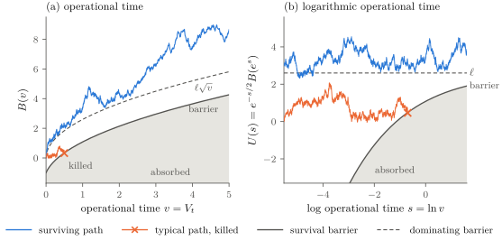
volatility path used in the lower bound, this barrier is a shifted square-root profile in the
operational time (Figure 2(a)). In the logarithmic time , the process is a stationary
Ornstein–Uhlenbeck process and the barrier becomes an essentially constant level (Figure 2(b)).
Holding above costs per unit of logarithmic time, over a window of length about . This
cost, to leading order, is of the same order as that of the volatility excursion, and the
two add up to . Equivalently, the effective volatility of volatility in the right wing is .
The absorbing boundary thus acts on the right tail through survival conditioning, not
through the mass at zero; the model-free tail-to-wing transfers [Lee04; BF09; GL14] are
unaffected.
Figure 2. Survival as a moving-barrier problem (; schematic simulation). (a) Along the exponential
volatility path, survival requires the orthogonal Brownian motion to stay above a shifted square-root
barrier in operational time ; a typical path is killed early. (b) In logarithmic time, is a stationary
Ornstein–Uhlenbeck process and the barrier rises to the constant level , which dominates it. The
lower-bound construction of Section 4 holds just above , at a cost of about per unit of .
Turning this mechanism into a proof requires matching bounds that do not presuppose path
concentration. For , the upper bound on (Section 3) drops the nonpositive singular drift, discretizes
the volatility excursion by level-hitting times, and converts the conditional survival constraints into a
finite-dimensional Cameron–Martin energy. A deterministic convex inequality (Lemma 3.7) then
bounds the total cost from below; its key step, Lemma 3.6, shows that the part of the Gaussian cost
that is linear in the displacement is minimized by deferring the displacement for as long as the
barrier allows. The matching lower bound (Section 4) combines a change-of-measure tube for
volatility with a Brownian path that enters and stays above the induced barrier, followed by a
bootstrap control of the singular drift. For (Section 5), a terminal-only upper bound is
paired with a lower-bound construction based on scale-invariant doubling and dyadic
level-raising steps. These arguments use elementary probability and finite-dimensional convexity
rather than a sample-path large-deviation principle, heat-kernel estimates or spectral
asymptotics.
1.4Relation to Prior Work
The problem lies at the intersection of several established theories, but not inside any one of their
proved regimes. Among the results we located, summarized in Table 1, none treats the
fixed-maturity extreme right wing of correlated SABR with . The closest results concern the
uncorrelated wing, the moment-explosion regime at , asymptotics of survival probabilities,
small-time geodesic expansions, and the left wing generated by the atom at zero. In particular,
Paulot [Pau15] cautions that small-time geodesic expansions are valid only as long as the geodesic
does not reach the boundary; the present result is a fixed-maturity, extreme-strike manifestation of
the same boundary obstruction.
Table 1. Selected results on extreme strikes and boundary effects for SABR-type models.
Before turning to the proofs, we record precisely what is proved. All limits are taken for fixed , and .
We do not prove uniformity in these parameters, a quantitative remainder, results at or , or a
left-wing theorem. No Dirichlet heat-kernel estimate is used or proved; Remark 6.3 describes
what such an estimate would have to provide. For we state a conjectural correction
(Conjecture 8.1), supported by formal calculations only; no proved result depends on it. The
numerical results of Section 7 illustrate the theorems and play no role in the proofs. Selected
deterministic steps have also been formalized in Lean; see the Supplementary Material
section.
Section 2 collects the reductions: the Lamperti decomposition, conditioning on volatility, and the
transfer to implied volatility. Sections 3 and 4 prove the upper and lower bounds for ; Section 5
treats and completes the proof of Theorem 1.1. Section 6 proves the intrinsic-distance identification,
Section 7 presents numerical illustrations, and Section 8 discusses the subleading correction and
neighbouring parameter regimes. Appendix A records measurability facts and Appendix B the
numerical methods.
2Preliminaries
The proofs rest on two reductions. The Lamperti–CEV transform isolates the correlation term and
lets us represent the orthogonal martingale in its quadratic-variation time; a model-free argument
converts logarithmic tail rates into implied-volatility limits.
Throughout, , , and are fixed, , and
so that . Constants depend only on the model parameters
and on the auxiliary parameters fixed in the current section, never on ; their values may change from
section to section. Upper and lower bounds always refer to .
2.1The Lamperti Decomposition
The first reduction is a change of coordinates. In the Lamperti coordinate the component driven by
the volatility Brownian motion integrates exactly, leaving an orthogonal Gaussian martingale and a
nonpositive singular drift.
Lemma 2.1 (Lamperti Decomposition).Let . There is an event with such that, for every and every with ,
where continuous versions are used throughout. Moreover, up to a null set; in
particular .
Proof.Apply Itô’s formula to the processes stopped at and let . With this gives before ,
using . Decompose and use , whence . Intersecting the full-measure events obtained at rational
stopping levels and using continuity yields one event on which the identity holds simultaneously
for every admissible . The event identity follows from the strict monotonicity of on and the
absorption convention, since on .∎
We write
for the process with the singular drift removed.
2.2Conditioning on Volatility: Operational Time
Conditioning on the volatility path completes the first reduction: the orthogonal martingale then
becomes a Brownian motion run on its quadratic-variation clock.
Lemma 2.2 (Conditional Brownian Time Change).Let be Wiener measure on , let denote the law
of the volatility path on , and for a continuous path put
There is a measurable regular conditional
distribution of the -valued random variable given such that, for -almost every volatility path ,
Equivalently, for such , let be the inverse of ; then has the standard Wiener law on
.
The jointly measurable versions and the kernel construction are recorded in Appendix A. We call
the operational time, write for the inverse quadratic-variation clock of the volatility path, and set
so that . By Lemma 2.2, conditionally on , is a standard Brownian motion on . “Conditionally on
the volatility path” always means evaluation under the kernel for -almost every path; the operational
times, thresholds and events entering such evaluations are measurable functions of the
path.
2.3Transfer to Implied Volatility
The second reduction is model-free: once the logarithmic tail rate is known, no further SABR
structure is needed to identify the right-wing limit. The forward is a nonnegative local martingale,
hence a supermartingale, so ; this is all the integrability we use. Write for the undiscounted call
price.
Lemma 2.3 (Tail-to-Implied-Volatility Transfer).If and for all sufficiently large , then .
Proof.(i) Prices. By the layer-cake identity (Fubini, using ), . Fix and with for . Substituting and
using , for large
Hence . Since , the implied volatility exists and is unique by strict monotonicity of
the Black–Scholes price in .
(ii) Black–Scholes tail. With and one has , hence , and the Mills bounds , , give
whence,
uniformly on compact -sets,
Only the leading term is used below; the bracketed constant follows
from the prefactor , and .
(iii) Identification of the limit. Suppose along a subsequence with . Pick ; eventually ,
contradicting . The case (including ) is symmetric. Hence .∎
By Lemma 2.3, Theorem 1.1 implies Corollary 1.2, and hence Corollary 1.3; the positivity
follows from the lower-bound constructions of Sections 4 and 5. Sections 3 to 5 prove
Theorem 1.1.
3Upper Bound for Negative Correlation
We begin with the upper bound on for negative correlation. This half of Theorem 1.1 must rule out
every cheaper way of producing the tail, including paths that raise the orthogonal component before
the barrier requires it.
Proposition 3.1 (Upper Bound, ).For ,
Conditionally on volatility, removing the nonpositive drift turns survival into a Brownian
moving-barrier event. We discretize the volatility excursion by level-hitting times, convert
each conditional event into a convex quadratic energy, bound the combined volatility and
boundary-crossing cost from below, and sum over the resulting configurations. Throughout this
section .
3.1Drift Removal
The singular drift is nonpositive before absorption. Dropping it enlarges the joint
survival-and-terminal event and isolates the Gaussian constraints that determine the upper
bound.
Lemma 3.2 (Drift Removal)..
Proof.On survival , so the drift is nonpositive and for all .∎
3.2A Gaussian Convex-Set Bound
At the level-hitting times introduced below, the relaxed survival and terminal requirements become
linear inequalities for a Gaussian vector. The following projection estimate converts their conditional
probability into a Cameron–Martin energy.
Lemma 3.3 (Gaussian Convex-Set Bound).Let be a centred Gaussian vector in , , with
symmetric positive definite covariance matrix , and let be nonempty, closed and convex with .
Then , where is the Mahalanobis distance and .
Proof.Write with standard Gaussian and . Let be the projection of onto , so that . The
supporting hyperplane at gives , and .∎
Apply the lemma to at -measurable operational times with thresholds and a terminal threshold
at . Put , , for , and . For define the extended-real increment energy
The constraint set is a
nonempty intersection of half-spaces, and the Markov structure of the Brownian covariance identifies
its squared Mahalanobis distance with the moving-barrier quadratic program
the Cameron–Martin
energy of the cheapest interpolation through the constrained nodes. In the applications
below for all sufficiently large , so the constraint set does not contain the origin. If , the
zero-increment convention forces ; this amounts to merging the coincident nodes with the single
threshold , and Lemma 3.3 is applied after this merge, so that its covariance matrix is
positive definite. The same formula with no intermediate nodes covers the terminal-only case
.
3.3Level-Hitting Skeleton
To retain sharp costs with finitely many constraints, we discretize the increase of log-volatility by
successive level-hitting times. The same skeleton controls the available quadratic variation,
the induced survival thresholds, and the probability of completing each level crossing
quickly.
Fix and set , (so ), , and . Along this skeleton the levels control the available quadratic
variation, and survival becomes a finite list of threshold conditions at the nodes.
Lemma 3.4 (Skeleton Constraints). (i) For every , ; hence
(ii) On one has for , and .
Proof.(i) is immediate from the definition of first passage; the cap on holds because
(ii) Since by
continuity and , the inequality reads , and reads .∎
Conversely, crossing a level quickly is costly for the volatility, as the reflection principle
shows.
Lemma 3.5 (Level-Hitting-Time Bound).On , for every ,
Consequently, for any thresholds , by
iterated conditioning,
Proof.By the strong Markov property, from the log-volatility runs as for a fresh Brownian
motion ; rising by within time forces , and the reflection principle gives the bound.∎
3.4Deferred Displacement and the Energy Inequality
The preceding reductions leave a deterministic question: can a path bring its combined volatility and
Gaussian cost below , by redistributing the volatility increase or by raising the Gaussian coordinate
before the barrier requires it? The next two lemmas show that it cannot. The key input is an
elementary summation-by-parts bound for the part of the Gaussian cost that is linear in the
displacement.
Lemma 3.6 (Deferred Displacement).Let and , write , and put . For all with for ,
with
equality for the maximally deferred choice .
Proof.Let and . Then and , so . Summation by parts with gives
since . For the increments
are nonnegative and both inequalities are equalities.∎
With this bound for the linear part, the combined volatility and Gaussian energy can be bounded
below uniformly over all allocations of time and quadratic variation.
Lemma 3.7 (Energy Inequality).For every and there are and , depending only on and the
model parameters, with the following property. For every and there is such that the estimate
below holds for every , every integer , and every admissible choice of increments.
Let with , let , and append a terminal increment , where . In (3.2) take the operational-time
increments , the thresholds of Lemma 3.4, and a terminal threshold with
Then
Proof. is nonincreasing in each operational-time increment, so we may replace by its upper
bound and the terminal increment by ; this remains valid when the actual terminal increment
is zero, because the convention in (3.2) is the lower-semicontinuous limit as that increment
decreases to zero. Write the QP variables through their increments () and , so that and
. Per interval,
and by Cauchy–Schwarz ; the terminal term is kept aside as a separate
nonnegative summand. Put . All -terms below are uniform in and in the admissible increments;
the coefficient of is uniform for small , and once are fixed the coefficient of does not depend
on .
Main case . Drop the terminal term. For any with , . The weights decrease and the
thresholds increase, so Lemma 3.6 gives
where continues the formula of Lemma 3.4; indeed
whenever . If denotes the level at which becomes nonnegative, then . Raising the Gaussian
coordinate earlier than the barrier requires can therefore only increase this sum. Hence
and
optimizing the direction, . With and ,
Case . Here for large . Since , either or . In the former case
in the latter, taking , , and
squaring gives at least . Both dominate for .
Finally choose and so that the loss in the main case is at most . For each fixed and ,
enlarge so that the loss is at most , , and the exponential bounds of the second case dominate
. This gives the factor uniformly over and all admissible increments.∎
The proof never identifies the minimizer of the aggregated functional, which is not obtained by
exact barrier tracking: the directional bound and Lemma 3.6 apply to all feasible allocations
simultaneously.
3.5Assembly
It remains to sum the cellwise bounds without losing the quadratic exponent. We first
remove exceptionally high volatility levels and very short passage times, then bin the
remaining passage times so that Lemma 3.7 applies uniformly at a combinatorial cost of only
.
Proof of Proposition 3.1. By Lemmas 2.1 and 3.2, . Fix in the ranges of Lemma 3.7; let , ,
, and define time bins for and .
(a) High volatility. , so by the reflection principle its probability is at most for large , since
.
(b) No level crossing, . Then on , , and the one-node case of Lemma 3.3 bounds the
conditional probability by .
(c) Configurations. For , partition according to the configuration and write the upper end of the
bin of as
where is the bin containing . If some , Lemma 3.5 alone bounds the probability by for
large . The number of configurations is at most , so these cells contribute at most . Otherwise , hence
, and on each cell the volatility cost is at most by Lemma 3.5 with thresholds , while the conditional
Gaussian cost is at most by Lemmas 3.3 and 3.4, with the operational-time increments bounded
through (larger increments decrease ). Their product is bounded by Lemma 3.7 with
.
(d) Sum. Combining,
Letting and then , with fixed admissible for each , proves the
proposition.∎
4Lower Bound for Negative Correlation
We now construct surviving paths that produce the tail at the rate , which gives the reverse
inequality.
Proposition 4.1 (Lower Bound, ).For ,
The construction separates the two leading costs. A Girsanov change of measure confines
volatility to a tube around an exponential path; conditionally on that tube, the orthogonal Brownian
motion enters and stays above the induced square-root barrier (Figure 2). A bootstrap then shows
that the chosen margins absorb the singular drift and imply the terminal event. Throughout this
section .
Fix , set and , and let . The exact identity shows that the exponential path is a shifted
square-root profile in its own quadratic-variation time.
4.1Volatility Tube
We first confine volatility near the exponential path suggested by the leading variational balance. The
logarithmic tube below has the unconstrained quadratic cost and distorts the volatility level and its
quadratic-variation clock only by fixed factors.
Lemma 4.2 (Volatility Tube).For and let and
Then
On , and for all .
Proof.Let , and let be the measure, given by Girsanov’s theorem, under which is a Brownian
motion. The extra absorbs the Itô term, so that exactly
Hence , and on , where ,
The bounds on
and are immediate.∎
With the lemma gives
4.2Target Event for the Orthogonal Component
Conditionally on a volatility path in the tube, the orthogonal Brownian motion must keep positive
before the barrier becomes active, stay above the moving barrier afterwards, and leave enough
terminal margin to reach once the singular drift is restored.
Let denote volatility in operational time. Set and let be the first operational time
at which exceeds ; since and is continuous, . Define
On the tube, with , the identity
and Lemma 4.2 give the two-sided bound
so the moving barrier is dominated by ,
where . Evaluating (4.2) at shows with , provided , which we assume henceforth. The
constants of this section may depend on the fixed , which is harmless because only after
.
4.3Bootstrap Control of the Singular Drift
The slack factors in were chosen to dominate the accumulated singular drift. The next
lemma turns the tube-and-barrier event into a surviving path that reaches the terminal
target.
Lemma 4.3 (Bootstrap).On , for all large (given ), and .
on the first branch , so , and on the second . Hence the drift
integral satisfies
so uniformly in . In particular throughout for large , which is incompatible
with . Hence on , that is, .
Terminal value. The terminal constraint in and the drift bound give, for large,
In the first
line the term cancels all but the -fraction of the barrier margin; in the second, because
.∎
4.4Barrier Tracking
It remains to show that has the required conditional probability. Under the logarithmic change of
operational time, a square-root Brownian barrier becomes a constant barrier for a stationary
Ornstein–Uhlenbeck process (Figure 2(b)). This representation does not control the initial entry, so
the construction first follows an explicit Cameron–Martin path segment and then concatenates
Ornstein–Uhlenbeck survival blocks.
Fix and , where is chosen so that on the tube (possible since and ). Set
Here and are
constants independent of , while . We use the constant barrier for only on , where , and bridge
explicitly. Two elementary lemmas isolate the probabilistic inputs.
Lemma 4.4 (Brownian Barrier Entry).Conditionally on a volatility path in the tube, for all
,
with .
Proof.Let be piecewise linear: on , rising linearly to at , and constant on . On all three constraints
hold: on , for large (as ); on , ; and . The localized Cameron–Martin shift along and Brownian
scaling, , give
since
on the localization event, while is a constant depending only on and the
parameters, and .∎
After the entry, the path is carried through blocks of logarithmic length between and ; the next
lemma gives the cost of a single block.
Lemma 4.5 (Ornstein–Uhlenbeck Survival Block).Let solve . For each there exist and such that for all , all durations , and all ,
Proof.Write and tilt the driving Brownian motion by the constant drift : under the tilt, is
an Ornstein–Uhlenbeck process centred at . The localized Cameron–Martin inequality applies
with and ; since and is at least standard deviations, the subtracted term is at most . For
the main term, the recentred process is a centred Ornstein–Uhlenbeck process started at , and
the event contains because for . That event contains the tube event with linear from to
. The law of the centred process on is a nondegenerate Gaussian measure with full support
on continuous paths from , so the tube probability is positive and depends continuously on ;
hence it is bounded below by some on that compact set. Therefore for .∎
Concatenating the entry segment with about such blocks yields the conditional probability of
.
Lemma 4.6 (Barrier Tracking).For every fixed and , conditionally on a volatility path in
the tube,
with as for fixed .
Proof.Domination. For one has , hence
while on the moving barrier is at most . In the
coordinate
a stationary Ornstein–Uhlenbeck process with covariance , the first event reads
Entry and block concatenation. Apply Lemma 4.4. Then, by the Markov property of at the
-measurable operational time and the Markov property of at the endpoints of blocks of equal
duration, where
Lemma 4.5—uniform over starting points in and over —applies at every block:
Since , and , all terms other than total .
The constructed event implies . On the intersection above, on and on (entry); on
(domination); and the terminal threshold holds because
for : the first summand dominates by (4.2),
and since . Hence the constructed event is contained in , and gives the claim.∎
4.5Assembly
The volatility-tube and conditional barrier-tracking costs add at the quadratic scale; all entry,
block-concatenation, localization and bootstrap terms are of lower order.
Proof of Proposition 4.1. By Lemmas 2.1 and 4.3, , and by Lemma 2.2, (4.1) and Lemma 4.6,
where we used
Let , then and , and use .∎
5Nonnegative Correlation
For nonnegative correlation the correlation term no longer creates a growing negative barrier, and the
rate is the unconstrained one. The upper bound therefore needs only a terminal Gaussian
constraint, while the lower bound must still control the singular drift. Throughout this section
.
5.1Upper Bound
Even after the survival constraint is dropped, no terminal strategy improves on the unconstrained
quadratic rate.
Proposition 5.1 (Upper Bound, ).For ,
Conditioning on volatility reduces the problem to a one-node Gaussian estimate coupled to the
level-hitting cost of Section 3. By Lemmas 2.1 and 3.2, dropping the survival constraint as well, ,
and conditionally on the volatility path the one-node case of Lemma 3.3 gives
We reuse the
level-hitting skeleton, the operational-time bounds, the time bins and the configuration count of
Section 3.5, with no running constraints and only the terminal node, and take . The
high-volatility tail then has probability at most and the cell at most , exactly as in
Section 3.5(a)–(b). The per-configuration estimate is the following terminal-only analogue of
Lemma 3.7.
Lemma 5.2 (Terminal-Only Energy).Fix , and . There are constants , depending only on
the model parameters, and such that for all , all , and all with ,
Proof.Set . Case 1: (possible only for ). Then
and Cauchy–Schwarz gives, for ,
the factor
absorbing the loss from . Case 2: otherwise. Then, for ,
so the terminal term is at least
If this is at
least ; if , Cauchy–Schwarz as in Case 1 gives
∎
The upper bound now follows by summing over configurations as in Section 3.5.
Proof of Proposition 5.1. Within each configuration, Lemma 3.4(i) gives on and hence
so the
product of the level-hitting cost (Lemma 3.5 at the thresholds ) and the conditional Gaussian
factor is bounded by Lemma 5.2 applied with and ; the second branch of the minimum
is superquadratic in . Summing over the configurations, letting and then proves the
proposition.∎
5.2Lower Bound
For the matching lower bound it suffices that survival and the terminal adjustment cost only beyond
the volatility excursion.
Proposition 5.3 (Lower Bound, ).For ,
We confine volatility near an exponential path whose endpoint is a fixed multiple of the target
level. The forward is then raised, first by scale-invariant doublings and then by dyadic
level-raising steps; both the orthogonal Brownian cost and the accumulated drift loss remain
subquadratic.
Parameters. Fix with . Let and choose a constant , depending only on the parameters, such that
with
one has . Unlike in Section 4, the terminal volatility is only a fixed multiple of . This keeps on
the tube, so that the singular drift accumulated during the level-raising and holding phases below is
only ; with an exponential overshoot , the drift accumulated at height would exceed that
level.
absorbed at its first zero. The equation is invariant
under the Brownian scaling
and two solutions driven by the same with ordered initial values
remain ordered up to the absorption of the lower one (the argument of Lemma 5.4 below
with ). The following lemma reduces survival of to survival of on the operational-time
horizon.
Lemma 5.4 (Comparison on the Operational-Time Horizon).Fix a volatility path in the
tube, and put and , so that
up to the first zero of . Let solve (5.3) on with and the same ,
and let . Then for . In particular, if then and .
Proof.The path is continuous but need not have finite variation; only the bound from (5.2)
is used. For and before any first crossing of ,
By continuity no crossing occurs, so on , and
the claims follow.∎
Starting from , the comparison process is first raised geometrically. By scale invariance, the
success probability of each doubling is bounded below independently of the level.
Proof.By Brownian scaling, the event has probability for every . On it, as long as the drift
integral is at most , so throughout ; hence there is no first passage below , and .∎
Doublings at the natural time scale can continue only up to the level , because the
operational-time budget is only of order . Above that level we force the remaining steps by a
Cameron–Martin shift, each certified by the following Gaussian estimate.
Lemma 5.6 (Brownian One-Step Lower Bound).Let with . Then .
Proof.Tilt by the drift . The localized Cameron–Martin inequality with gives . Under the tilt
, which has probability at least by the reflection principle; and , so the subtracted term equals
. Since , the claim follows.∎
For the forced steps let , and define the nominal levels for and , so that the last ratio lies
in . With , allocate the operational-time increments to the steps ; since , they total at
most . Over these steps the process climbs from to at an exponential cost of order
only.
Lemma 5.7 (Level Raising).There is such that the following holds for , conditionally on
a volatility path in the tube. Let solve (5.3) with , and let . With probability at least , stays
positive on and ; along the way its total drift loss is .
Proof.Restart the comparison at the nominal levels: a solution entering step at a value at least
dominates the solution started at , so it suffices that the latter reach within . Apply Lemma 5.6
with , and . On the tube , hence, uniformly in ,
for , so each step certificate has probability at least
On the certificate the bootstrap of Lemma 5.5 applies: the drift loss during the step is at most
since
. Hence throughout the step, and at its end
The certificates concern Brownian increments over
disjoint intervals, so their probabilities multiply. The costs are
and the total drift loss is at most
.∎
Once the level is reached, keeping the process above until the horizon is nearly free.
Lemma 5.8 (Holding).Fix a volatility path in the tube and a -measurable operational time ,
and suppose . Let
Then , which tends to one uniformly over the tube and over ; and on , for large, stays positive on and .
Proof.The formula is the reflection principle, and it is at least . On the tube,
For the drift,
bootstrap once more: let . On the drift integral is at most , while on the decrease of is at
most ; hence up to , so , and the same bounds give .∎
The three phases, doubling, level raising and holding, combine to give the lower bound.
Proof of Proposition 5.3. Fix a volatility path in the tube. By Lemmas 2.1 and 5.4, it suffices
to show that, with conditional probability at least , the solution of (5.3) with stays positive
on and satisfies . We combine three phases by the Markov property at their -measurable
endpoints.
Doubling. Apply Lemma 5.5 at the dyadic levels from up to : there are stages, each
starting no lower than its nominal level by the ordering of solutions of (5.3). They succeed
together with probability at least and use operational time at most , by the choice of .
Level raising. Lemma 5.7 raises from at least to at least within further operational time
, with probability at least .
Holding. The level-raising phase ends at an operational time ; by Lemma 5.8 the conditional
probability that then stays positive and ends above tends to one.
Multiplying the three conditional bounds and integrating over the tube with (5.1) gives
The four propositions combine to give the main theorem and its corollaries.
Proof of Theorem 1.1. For the theorem is Propositions 3.1 and 4.1; for it is Propositions 5.1
and 5.3. The lower-bound constructions show for all large , so Lemma 2.3 applies and yields
Corollaries 1.2 and 1.3. At this recovers [BFL08].∎
6The Intrinsic Distance in the Survival Domain
We now prove the geometric identification (1.4). Henry-Labordère’s derivation of (10.22) in [Hen08]
represents the SABR generator by a Riemannian metric, a connection and a scalar potential
on a patch of the Poincaré half-plane, and then uses a Gaussian estimate based on the
unrestricted geodesic distance. For the absorbed model the correct leading quantity is
instead the intrinsic distance within the open survival domain, the state space of the
process killed at the boundary. The calculation below is elementary and uses no heat-kernel
theorem.
6.1Fermi Coordinates and the Survival Domain
The hyperbolic geometry of SABR is most transparent in Fermi coordinates around a geodesic, in
which the survival domain becomes the coordinate half-plane , bounded by a curve at constant
distance from that geodesic. Recall , and set
Before absorption, and are driven by the independent
Brownian motions and with the common volatility , so the principal symbol of the generator is that
of the hyperbolic metric . In the coordinates ,
and the open survival domain and the metric are
Thus is the signed distance from the geodesic , and motion in at fixed costs per unit of
.
Distances in are measured along paths that stay in . For , let be the class of finite chains , , of
legs with , and . Every leg respects the domain constraint, while minimizing sequences may
approach the boundary. For set
and for . Let be the initial point, so that and , and let
be the
terminal target set.
6.2The Distance to the Target Set
Reaching requires a displacement of about in , and such motion is cheapest where is smallest. The
distance is therefore governed by the infimum of over .
Proposition 6.1 (Intrinsic Distance to the Target Set).Let , that is, for and for . Then, as ,
For the bound is approached by curves whose long tangential segment tends to the absorbing
boundary; for the minimizing tangential line lies in the interior.
Proof.Since , one has precisely when . As and are unit vectors, on . Hence every satisfies
Moreover : if , then and the infimum is (approached from within when ); if , then and the
infimum is . Therefore every admissible chain from to satisfies, for all sufficiently large ,
For
the reverse bound, first let . The three-segment path
stays in , ends in , and has length . If ,
set . For all sufficiently large the analogous path through stays in , has the same endpoint ,
and has length
Returning to the fixed level makes the terminal constraint exact and avoids
the displacement that would arise if the endpoint stayed in the boundary layer.∎
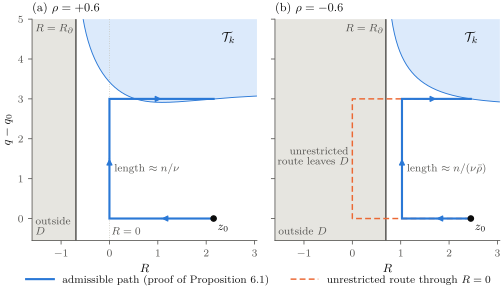
Figure 3. Fermi coordinates for the reference parameters of Section 7 with and . The survival domain
is ; the shaded strip lies outside , and is the target set. Motion in costs per unit, least on the line
. (a) For the line lies in , and the paths of the proof of Proposition 6.1 have length , as in the
unrestricted metric. (b) For the line lies outside ; admissible paths can only approach the boundary,
where the cost is , so the distance grows like .
Combined with Theorem 1.1, the proposition identifies the tail rate with the intrinsic distance.
This is the corrected form of Conjecture 2 for the absorbed model.
Corollary 6.2 (Corrected Conjecture 2 for Absorbed SABR).For every ,
Proof.By Proposition 6.1, , which equals by Theorem 1.1.∎
6.3Unrestricted versus Intrinsic Distance
The comparison with the unrestricted distance shows exactly where the Gaussian estimate behind
Conjecture 2 breaks down. Let denote the distance to the same set when connecting curves may
range over the whole Fermi plane. The lower-bound and three-segment arguments above give for
every : the unrestricted plane always permits the long segment on . If , however, and the line lies
outside ; admissible curves can only approach , where the tangential cost is (Figure 3). If the line is
interior, and if it is the boundary but can be approached without changing the leading coefficient.
Thus the intrinsic and unrestricted distances agree to leading order exactly when the excluded region
is irrelevant on the scale. Paulot [Pau15] pointed out the corresponding boundary restriction
on small-time geodesic expansions; Proposition 6.1 is its fixed-maturity, extreme-strike
analogue.
6.4The Potential Is Unbounded on the Survival Domain
The endpoint value in Conjecture 2 does not control the lower-order part of the operator. In the
Lamperti–CEV coordinate the full scalar potential is
which has an inverse-square singularity at the
absorbing boundary. For the unrestricted saddle on the fibre , with and , the exact formula [Hen08,
(6.45)] is
Thus as , which gives (1.2) and shows that the potential remains bounded along the
far-right saddle, although its finite-strike value is generally not constant. Moreover, in
Henry-Labordère’s convention the connection one-form is
which is singular and, for , not globally gauge-removable. These terms do not affect Corollary 6.2, but the formal calculation of Section 8.1
indicates that they contribute at order . They are also the obstacle to a heat-kernel proof of
Corollary 6.2.
Remark 6.3 (A Heat-Kernel Route). A Dirichlet heat-kernel theorem would give a second route to
(6.3), closer to Henry-Labordère’s method. Let be the Dirichlet heat kernel of the generator on —the
transition density of the killed process—with respect to a reference measure , so that .
It would suffice to prove
uniformly on a subset with
together with an exponentially
matching bound for the integral over , for instance a global upper estimate with subquadratic
logarithmic volume factors. Gaussian bounds of Li–Yau type [LY86; Dav89; Stu92] do not apply
directly, because the potential and the connection are singular at ; whether a suitable
singular-potential framework applies is open. The proofs in this paper establish both tail inequalities
directly.
7Numerical Illustrations
The theorems concern leading rates, which finite-strike computations can illustrate but not establish.
We report Monte Carlo estimates of at moderate strikes, which display the correlation
asymmetry, and solutions of the deterministic variational problems behind the two rates up to .
Methods are summarized in Appendix B. All computations use , , , , and , for which
Table 2. Monte Carlo estimates of with delta-method standard errors. : effective sample size below ;
these errors should be read with caution.
2
—
—
3
—
—
4
5
—
—
6
8
—
—
10
—
—
—
12
—
—
—
At these strikes the asymptotic regime is still distant: at , the implied volatility is only
about at , against the limit . Table 2 therefore cannot be read as a rate. The correlation
asymmetry is nevertheless visible in the spreads
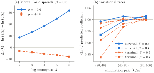
for which Theorem 1.1 gives and . In
Figure 4(a), is close to linear in (its second differences at unit spacing are within of
zero), while is convex, with second differences between and . These exceed the value
contributed by the term alone, consistent with the positive correction of Conjecture 8.1; the
window is too short to separate the two, and we draw no quantitative conclusion from
it.
Figure 4. (a) Monte Carlo spreads at from Table 2, with standard-error bars (marginal errors
combined in quadrature; mostly smaller than the markers). The spread for is close to linear, consistent
with equal coefficients for and (Theorem 1.1 gives ); the spread for is convex. (b) Eliminated
coefficients of Table 3, divided by their predictions: for the survival problems () and for the terminal
problems ().
Variational Rates. The logarithmic rates are governed by deterministic control problems: minimize the
Cameron–Martin energy of the volatility driver plus the Gaussian energy of the orthogonal
component, subject to the terminal constraint (the terminal problem) or to the terminal and survival
constraints (the survival problem); see Appendix B. Their values , normalized by , are predicted to
approach , and for the survival problem with . We solve them for and remove a term
linear in by the elimination
At the pair every estimate lies within of its prediction
(Table 3 and Figure 4(b)). The individual coefficients depend on through ; the -independent
prediction is the ratio , against which the survival-to-terminal ratios at are for and for
.
Table 3. Eliminated quadratic coefficients of the variational problems, from the pairs with .
problem
prediction
survival
0.5
0.5381
0.5498
0.5458
terminal
0.5
0.3347
0.3488
0.3522
terminal
0.5
0.3412
0.3470
0.3474
terminal
0.5
0.3430
0.3463
0.3470
survival
0.7
0.1825
0.1940
0.1981
terminal
0.7
0.1047
0.1210
0.1260
terminal
0.7
0.1139
0.1227
0.1248
Checks of Analytic Ingredients. We also tested several formulas and implementations numerically: the Gaussian convex-set bound
of Lemma 3.3 by -path Monte Carlo on a three-node instance; the functional of Lemma 3.7 in the
limit by exhaustive minimization over at , which gives normalized minima , and at , consistent
with the slack factor of that lemma, and starts with early Gaussian displacement converge to the
same minima; the block probabilities of Lemma 4.5 at ; the doubling and level-raising certificates of
Section 5.2 on a time grid; the expansion (2.3) up to ; and the Ornstein–Uhlenbeck eigenvalue
computations of Section 8.1, including the exact value . These checks are not part of the
proofs.
8Discussion
We close with two complementary perspectives on the main theorem: what lies beyond the leading
order when , and how the absorbed model sits between the neighbouring regimes and
.
8.1Beyond the Leading Order
Theorem 1.1 settles only the leading scale. For four statements of different status must be kept
apart: the square-root-boundary eigenvalue expansion below is classical for the drift-free comparison
process; the Fourier–Laplace reduction of the full generator with Dirichlet boundary condition is
exact; the ensuing boundary-layer localization and Legendre inversion are formal; and the resulting
correction is conjectural.
Along the leading exponential volatility excursion, dropping the singular drift from the
survival constraint gives the moving-barrier comparison problem . Under , is a stationary
Ornstein–Uhlenbeck process constrained to stay above , with survival exponent given by the principal
Dirichlet eigenvalue on ; this is the square-root-boundary theory of Breiman [Bre67] and
Uchiyama [Uch80]. Its classical large- expansion is
where is the first zero of the Airy
function. The leading term reproduces . The Airy term is valid for the comparison problem,
but it cannot be transferred to the full SABR diffusion without restoring the singular
drift.
The exact lower-order obstruction appears after a transform in the tangential variable. In the
coordinates of Section 6, with
the backward generator on , with Dirichlet boundary condition at , is
All coefficients and the boundary are invariant under translation in . A real Fourier mode yields a
non-self-adjoint fibre; positive -displacement leads instead to the bilateral Laplace mode ,
equivalently the complex Fourier parameter . After conjugation by the radial speed measure,
the analytically continued fibre is a real one-dimensional differential expression with the intended Friedrichs realization. For and , its boundary expansion, shifted by the quadratic
maximum, is
The term is the singular tangential component of the drift. Balancing
it with gives
A formal one-dimensional min–max localization, with a bump of width
about , predicts the tilted principal-eigenvalue scaling
We do not prove (8.3): a proof
must specify the quadratic-form domain, establish the relevant discrete eigenvalue, and
supply a global localization upper bound. The inverse-square term is only at this scale but
formally selects the Dirichlet Friedrichs realization. At the ordinary Airy scale the term is
of order and dominates the Airy balance; within this formal balance the Airy regime
survives only in the driftless case , or for the comparison process without the singular
drift.
Formal Legendre inversion of (8.3), and a second, likewise formal, calculation that conditions
on the autonomous angular path and optimizes its exact Gaussian tail, give the same
prediction.
Conjecture 8.1 (Singular-Drift Subleading Correction).For and ,
A proof would require a uniform shrinking-tube lower bound or, alternatively, complex
saddle-point estimates controlling endpoint overlaps and transverse frequencies. The numerical
window of Section 7 cannot distinguish the term reliably from other corrections.
8.2Neighbouring Parameter Regimes
The geometry above identifies absorption, rather than correlation alone, as the source of
the negative-correlation correction. The neighbouring regimes are therefore informative:
the correlation structure persists, but the state space, and with it the tail mechanism,
changes.
At there is no absorption. Forde and Zhang [FZ15] show that the right tail for is governed by
the critical moment [LM07], with a one-sided discontinuity at ; the implied-volatility
smile grows rather than approaching a finite right-wing limit, consistently with Lee’s
moment formula [Lee04]. For , by contrast, moments of every positive order are finite
as a consequence of the quadratic log-moneyness tail proved here, and the right-wing
limit is finite; its value is but not at (Corollary 1.3). The same factor thus appears
in the two regimes through distinct mechanisms: moment explosion at , absorption at
.
The normal SABR model supplies the complementary boundary case. Its state space is all of
and it has no absorbing boundary; its right-wing limit is for every [Hen08, Example 10.4]. The limit
in Corollary 1.2, however, retains the factor , because it approaches through models that still have
an absorbing boundary at . The difference is caused by the change of state space, not by the CEV
exponent alone.
Finally, the mass-at-zero literature [GHJ18; DHJ17; Gul15] describes how the atom at the origin
shapes the left wing. Theorem 1.1 and Corollary 1.2 show that for negative correlation the same
boundary also changes the right-wing limit, acting through the survival constraint rather than
through the size of the atom. Taken together, these regimes show that the diffusion metric
alone does not determine the extreme wing: its interaction with the survival domain is
decisive.
AMeasurability, Versions and Uniqueness
This appendix records the measurability and well-posedness facts used when conditioning on a
volatility path, passing to operational time, and summing level-hitting configurations; it introduces
no additional probabilistic estimate.
(i) On every compact subset of the coefficients of the equation are locally Lipschitz. Standard
localization therefore gives a pathwise-unique strong solution up to , and the model convention fixes
its continuation by after . We use continuous adapted versions throughout. The stopped Itô
identities at levels , , hold simultaneously outside one null set; continuity then gives the all-times
formulation of Lemma 2.1.
(ii) The volatility path space is Polish. For a fixed continuous positive path , the Itô integral
with deterministic integrand is a centred continuous Gaussian process with covariance
. Since is -measurable, independence of and implies independence of and , and the
deterministic-integrand stochastic-integral theorem gives, for -almost every , the conditional path law
as stated in Lemma 2.2 [KS91, Ch. 3]. The map is Borel measurable for the compact-open
topologies, so is a measurable probability kernel. Regular conditional distributions are unique
only -almost everywhere, and every conditional assertion in the paper is made with that
qualification.
(iii) Since for -almost every path, is and strictly increasing; its inverse is , and under the kernel
above has Wiener law on the finite random interval . In particular, the comparison statements of
Section 5.2 are confined to this operational-time horizon.
(iv) The level-hitting times are stopping times of the continuous adapted process , and all
skeleton data (, , and bin memberships) are -measurable. After coincident operational-time nodes are
merged, the QP in (3.2) is the minimum of a finite-dimensional coercive convex functional
over a closed polyhedron and is a Borel function of its operational-time and threshold
data. The conditional applications of Lemma 3.3 and the tower property are therefore
legitimate.
BNumerical Methods
This appendix summarizes the methods behind Section 7.
Monte Carlo estimators. We write , where is the conditional probability of the target event given
the volatility path. Volatility paths are sampled from a finite mixture of exponentially tilted path
measures and reweighted by the mixture likelihood ratio. Except for , , is estimated by an Euler scheme in operational time with antithetic inner draws and the drift-free Brownian-bridge correction
when both endpoints of a step are positive. The inner Brownian increments are tilted toward the
terminal target, by a constant tilt or by an equal mixture of a constant and a variationally scheduled
tilt, on grids of to steps. For , the inner probability is exact: conditionally on the volatility path, is
a squared Bessel process of dimension in operational time, absorbed at , so that with and
,
where is the regularized upper incomplete gamma function. The series is truncated
adaptively, with analytic bounds on the omitted Poisson tail that are negligible relative to
the estimate and its Monte Carlo error; independent Bessel-density quadrature agrees to
relative error , and the remaining discretization is the trapezoidal evaluation of on a -step
grid.
The reported errors are first-order delta-method standard errors of ; the second-order correction
is at most . Effective sample sizes are for importance weights ; the threshold for was chosen after
the runs. The cell pools two batches of paths. Grid-refinement ladders with , , and steps at the
representative cells , and bound the production-grid bias in by , and (two standard errors). They
do not bound the bias of the other cells; the sources of discretization error are the trapezoidal
integrated variance, the Euler treatment of the singular drift, and the drift-free bridge correction on
steps with drift.
Variational problems. With the volatility driven by a control , , operational time and correlation
term , the survival problem is
where the inner minimum is over paths with , , and for
all ; the terminal problem omits the last constraint. (The Itô correction in is of lower
order and is omitted.) We take piecewise linear on control nodes, interpolated on a -step
grid with exact operational-time increments on each step. With the survival constraint
imposed at the grid nodes, the inner problem is solved exactly: its minimizer is the least
nondecreasing concave majorant of the constraint points, anchored at the origin. The free terminal
value imposes a nonnegative final slope. We compute the ordinary concave upper hull and
replace its nonpositive-slope terminal portion by a constant continuation; equivalently, only
positive-slope segments contribute to the energy. The outer minimization uses L-BFGS-B followed
by Nelder–Mead from several initializations, with continuation in ; the computation is
deterministic. An earlier implementation, which imposed the inner constraints by penalties, gives
consistent but less regular elimination sequences; both are included in the supplementary
material.
Reproducibility. The supplementary material contains the scripts, the stored outputs and a
cell-by-cell provenance record. Not every displayed Monte Carlo value can be regenerated from a
recorded seed; the record states which can. For , , Table 2 reports a run with recorded seeds; an
earlier production run agrees with it to within in .
Supplementary Material
The supplementary material, available from the authors on request, contains the code and data for
Section 7 and the figures, and a Lean development. The Lean development formalizes the
fixed-volatility Black–Scholes call-price rate, the identification of the implied-volatility limit from a
call-price rate, and the intrinsic-distance calculation of Proposition 6.1, and derives Corollary 6.2
from that proposition with the two tail bounds as hypotheses. It states the stochastic inputs of the main proof as explicit interfaces and is not a formal proof of Theorem 1.1. A claim manifest links
statements of this paper to Lean declarations.
Acknowledgments and Tool Disclosure. The authors used OpenAI Codex and Anthropic’s Claude for language editing, restructuring of the
exposition, preparation of figures, and assistance with the supplementary Lean development and
computational checks. The authors take full responsibility for the mathematical claims, exposition,
code and numerical results.
Notes
The book writes the right-hand side of (1.2) as a constant value; the finite-point potential and saddle formula
in Section 6.4 give the large-strike limit stated here. Both conjectures appear on p. 306 of [Hen08]. Conjecture 1 is
stated there without restriction on and is immediately followed by the attribution of the case to [BFL08] (the book’s
reference [55]), which fixes its intended generality. ↩
References
[AP07]Leif B. G. Andersen and Vladimir V. Piterbarg. “Moment Explosions in Stochastic Volatility Models”. In: Finance and Stochastics 11.1 (2007), pp. 29–50. doi: 10.1007/s00780-006-0011-7.
[AKS13]Alexandre Antonov, Michael Konikov, and Michael Spector. “SABR Spreads Its Wings”. In: Risk (Aug. 2013), pp. 58–63.
[AKS19]Alexandre Antonov, Michael Konikov, and Michael Spector. Modern SABR Analytics. SpringerBriefs in Quantitative Finance. Cham: Springer, 2019. doi: 10.1007/978-3-030-10656-0.
[AS12]Alexandre Antonov and Michael Spector. Advanced Analytics for the SABR Model. SSRN preprint 2026350. 2012. doi: 10.2139/ssrn.2026350.
[BF09]Shalom Benaim and Peter Friz. “Regular Variation and Smile Asymptotics”. In: Mathematical Finance 19.1 (2009), pp. 1–12. doi: 10.1111/j.1467-9965.2008.00354.x.
[BFL08]Shalom Benaim, Peter Friz, and Roger Lee. “On Black–Scholes Implied Volatility at Extreme Strikes”. In: Frontiers in Quantitative Finance: Volatility and Credit Risk Modeling. Ed. by Rama Cont. Hoboken, NJ: Wiley, 2008, pp. 19–45. doi: 10.1002/9781118266915.ch2.
[Bre67]Leo Breiman. “First Exit Times from a Square Root Boundary”. In: Proceedings of the Fifth Berkeley Symposium on Mathematical Statistics and Probability. Vol. 2.2. Berkeley: University of California Press, 1967, pp. 9–16. doi: 10.1525/9780520325340-004.
[CY19]Nan Chen and Nian Yang. “The Principle of Not Feeling the Boundary for the SABR Model”. In: Quantitative Finance 19.3 (2019), pp. 427–436. doi: 10.1080/14697688.2018.1486037.
[Dav89]E. Brian Davies. Heat Kernels and Spectral Theory. Vol. 92. Cambridge Tracts in Mathematics. Cambridge: Cambridge University Press, 1989. doi: 10.1017/CBO9780511566158.
[DHJ17]Stefano De Marco, Caroline Hillairet, and Antoine Jacquier. “Shapes of Implied Volatility with Positive Mass at Zero”. In: SIAM Journal on Financial Mathematics 8.1 (2017), pp. 709–737. doi: 10.1137/14098065X.
[DHT17]Leif Döring, Blanka Horvath, and Josef Teichmann. “Functional Analytic (Ir-)Regularity Properties of SABR-Type Processes”. In: International Journal of Theoretical and Applied Finance 20.3 (2017), p. 1750013. doi: 10.1142/S0219024917500133.
[FP13]Martin Forde and Andrey Pogudin. “The Large-Maturity Smile for the SABR and CEV–Heston Models”. In: International Journal of Theoretical and Applied Finance 16.8 (2013), p. 1350047. doi: 10.1142/S0219024913500477.
[FZ15]Martin Forde and Hongzhong Zhang. “Sharp Tail Estimates for the Correlated SABR Model”. Preprint, King’s College London and Columbia University. Nov. 2015.
[GL14]Kun Gao and Roger Lee. “Asymptotics of Implied Volatility to Arbitrary Order”. In: Finance and Stochastics 18.2 (2014), pp. 349–392. doi: 10.1007/s00780-013-0223-6.
[Gul15]Archil Gulisashvili. “Left-Wing Asymptotics of the Implied Volatility in the Presence of Atoms”. In: International Journal of Theoretical and Applied Finance 18.2 (2015), p. 1550013. doi: 10.1142/S0219024915500132. arXiv: 1311.6027.
[GHJ16]Archil Gulisashvili, Blanka Horvath, and Antoine Jacquier. “On the Probability of Hitting the Boundary for Brownian Motions on the SABR Plane”. In: Electronic Communications in Probability 21 (2016), Paper No. 75. doi: 10.1214/16-ECP26.
[GHJ18]Archil Gulisashvili, Blanka Horvath, and Antoine Jacquier. “Mass at Zero in the Uncorrelated SABR Model and Implied Volatility Asymptotics”. In: Quantitative Finance 18.10 (2018), pp. 1753–1765. doi: 10.1080/14697688.2018.1432883.
[HKLW02]Patrick S. Hagan, Deep Kumar, Andrew S. Lesniewski, and Diana E. Woodward. “Managing Smile Risk”. In: Wilmott Magazine (Sept. 2002), pp. 84–108.
[Hen08]Pierre Henry-Labordère. Analysis, Geometry, and Modeling in Finance: Advanced Methods in Option Pricing. Chapman & Hall/CRC Financial Mathematics Series. Boca Raton, FL: Chapman & Hall/CRC, 2008. doi: 10.1201/9781420087000.
[KS91]Ioannis Karatzas and Steven E. Shreve. Brownian Motion and Stochastic Calculus. 2nd ed. Vol. 113. Graduate Texts in Mathematics. New York: Springer, 1991.
[Lee04]Roger W. Lee. “The Moment Formula for Implied Volatility at Extreme Strikes”. In: Mathematical Finance 14.3 (2004), pp. 469–480. doi: 10.1111/j.0960-1627.2004.00200.x.
[LY86]Peter Li and Shing-Tung Yau. “On the Parabolic Kernel of the Schrödinger Operator”. In: Acta Mathematica 156 (1986), pp. 153–201. doi: 10.1007/BF02399203.
[LM07]Pierre-Louis Lions and Marek Musiela. “Correlations and Bounds for Stochastic Volatility Models”. In: Annales de l’Institut Henri Poincaré C, Analyse non linéaire 24.1 (2007), pp. 1–16. doi: 10.1016/j.anihpc.2005.05.007.
[Pau15]Louis Paulot. “Asymptotic Implied Volatility at the Second Order with Application to the SABR Model”. In: Large Deviations and Asymptotic Methods in Finance. Ed. by Peter K. Friz, Jim Gatheral, Archil Gulisashvili, Antoine Jacquier, and Josef Teichmann. Vol. 110. Springer Proceedings in Mathematics & Statistics. Cham: Springer, 2015, pp. 37–69. doi: 10.1007/978-3-319-11605-1_2. arXiv: 0906.0658.
[Stu92]Karl-Theodor Sturm. “Heat Kernel Bounds on Manifolds”. In: Mathematische Annalen 292.1 (1992), pp. 149–162. doi: 10.1007/BF01444614.
[Uch80]Kôhei Uchiyama. “Brownian First Exit from and Sojourn over One Sided Moving Boundary and Application”. In: Zeitschrift für Wahrscheinlichkeitstheorie und Verwandte Gebiete 54.1 (1980), pp. 75–116. doi: 10.1007/BF00535355.
[YW18]Nian Yang and Xiangwei Wan. “The Survival Probability of the SABR Model: Asymptotics and Application”. In: Quantitative Finance 18.10 (2018), pp. 1767–1779. doi: 10.1080/14697688.2017.1422083.
How to cite
Zeyu Cao and Shaosai Huang (2026). The Right Wing of the SABR Smile with an Absorbing Boundary: Resolution of Conjectures of Henry-Labordère. Working paper, version of October 2026. Kspectra Research. SSRN 7562378 (doi:10.2139/ssrn.7562378); arXiv:2610.04209. https://kspectra.ai/papers/sabr-right-wing-absorbing-boundary/
@misc{cao2026right,
  author        = {Cao, Zeyu and Huang, Shaosai},
  title         = {{The Right Wing of the SABR Smile with an Absorbing Boundary: Resolution of Conjectures of Henry-Labordère}},
  year          = {2026},
  month         = oct,
  note          = {Working paper, version of October 2026},
  doi           = {10.2139/ssrn.7562378},
  eprint        = {2610.04209},
  archiveprefix = {arXiv},
  url           = {https://kspectra.ai/papers/sabr-right-wing-absorbing-boundary/}
}