Finite-factor term-structure models assign no independent risk to exposures between their factors, although desks treat them as risks of their own. The cylindrical term-structure model of [13] gives each maturity an independent shock, but specifies real-world dynamics, leaving the link to arbitrage pricing open. This paper settles that question for every finite truncation of the deformation at fixed spread intensity, and then restores the stochastic spread in two conventions. The key observation is that the deformation’s damped sine modes are imaginary parts of complex exponentials, so the smallest shift-invariant family containing them is a doubled sine–cosine envelope whose added coordinates carry no noise. On this envelope, whether the factor drift is arbitrage-free reduces to one polynomial divisibility, which the model’s maturity diffusion fails on every mode. Because the failure sits in the noiseless coordinates, no change of measure removes it. No such truncation admits an equivalent martingale measure; for generic maturities an explicit arbitrage uses one bond more than there are modes; and the defect grows with resolution. Giving those coordinates noise of their own turns the impossibility into a market price of risk that diverges with resolution. Adjoining those coordinates, keeping the model’s noise and correcting only the drift makes every truncation arbitrage-free. The required convexity has an exact limit under refinement, with a short-end jump resolved in a boundary layer at the resolution scale. Bond-level volatilities converge, but forward-curve distributions do not: within this construction, maturity-local noise, no-arbitrage at every resolution and a curve-valued limit cannot coexist. The short-end value survives the stochastic spread. It is conserved at every vol-of-vol in the uncorrelated affine convention, and recovered at zero vol-of-vol in the bilinear quadratic–Gaussian convention under a recovery normalization, where each truncation has an exact existence criterion. The consistency test and the arbitrage construction extend beyond this model.
A finite-factor term-structure model assigns no independent risk to exposures that fall between its
factors. For a symmetric butterfly, the modelled exposure is only the second difference of
smooth factor loadings, so it vanishes quadratically as the wings are brought in towards
the centre maturity. Desks nevertheless hedge and charge for the position as though it
carried local risk of its own. In practice, this gap is managed rather than eliminated.
Factor truncation, tenor buckets, proxy hedges, convexity overlays and basis-risk reserves
make a finite production system workable. They are operational accommodations: they
do not specify how the residual maturity risk should enter a common dynamic pricing
model.
Turning that residual-risk problem into a production pricing model requires answers to two
separate questions. Finite implementation asks what a finite truncation preserves and what depends
on its maturity resolution. Pricing consistency asks whether deterministic maturity roll-down and the
Heath–Jarrow–Morton (HJM) convexity drift remain inside the volatility span, so that the truncation
admits an equivalent local martingale measure. The first question concerns representation; the second
concerns no-arbitrage.
The cylindrical method [13] addresses the risk representation first: one innovation is assigned to
each maturity, rather than imposing smooth interpolation across neighbouring tenors. Write for time
to maturity up to the maximum modelled maturity . The forward curve is carried by a
deformation field ,
with a short rate, a scalar stochastic spread and a deterministic
shape, and solves the second-order stochastic evolution equation
Here transports the
curve as calendar time passes, diffuses shocks along the maturity axis at scale . The
noise is a cylindrical Brownian motion on of intensity : one independent innovation
per maturity, which is the whole point of the construction. The Dirichlet realisation of
that generator has orthonormal eigenbasis
with eigenvalues , so the coordinates are
independent Ornstein–Uhlenbeck processes reverting at rate . Each is a damped sine of
maturity frequency and common damping scale . Equivalently, it is the imaginary part of a
complex exponential with exponent : the real sine–cosine pair carries the conjugate pair, and
forward rates and bond prices remain real. These shapes belong to the class associated
with finite-dimensional arbitrage-free realisations [6, 19]. The dynamics, however, are
specified under the real-world probability measure , while the link to the risk-neutral pricing
measure is left open. With the spread held fixed, the link cannot be supplied as written: no
finite sine truncation of the deformation admits an equivalent local martingale measure
with its own volatility. That is the problem solved first; §6 then restores the stochastic
spread.
We call the cylindrical deformation field and the displayed specification the source model.
Unqualified, “the model” means the source model. In §§3–5, where the spread is held fixed, it means that model’s deformation sector, truncated to its first sine modes. “The completion” means the
arbitrage-free construction of §5; each stochastic-spread family is named by the assumption and
convention that defines it.
What makes the question answerable. To carry the analysis past the point at which
the link to was left open we start from the standard route: consistency is decided on
finite-dimensional shift-invariant families of curve shapes [6, 7, 19], in the invariant-manifold form of
[21]. Here that route is compulsory rather than convenient. Under cylindrical noise the
forward rate at a fixed maturity is not a semimartingale (§3), so the drift condition cannot
be posed maturity by maturity at all. On the curve the comparison is not merely hard
but ill-posed; finite-dimensional invariant subspaces are where the question can be made
rigorous.
The route is blocked at its first step. It asks for a shift-invariant family, and the model has none.
Its sine modes span no invariant space, so there is nothing for the realisation machinery to act on —
which is where the matter had rested.
The block dissolves once the spectrum is read as complex. Each mode is the imaginary part of . A
conjugate pair admits no one-dimensional real invariant subspace, so the smallest invariant space
containing one mode is two-dimensional. The model’s span therefore completes to the -dimensional
sine–cosine envelope, and it is on that envelope — not on the model’s own state space — that the
comparison can be made. This is the step the rest of the paper rests on, and it pays twice over. It
supplies the invariant family the standard route was asking for. And the coordinates it adjoins carry
no noise, while the missing rotation acts precisely on them: what would have looked, on the model’s
own span, like a correctable disagreement about drift is revealed as an obstruction that no
change of measure can remove. Complexification is the mechanism here, not a change of
notation.
The remaining steps follow from the envelope. On it the deformation and the arbitrage-free
transport both act by matrices, so the comparison of drifts becomes algebra. A generator
with symbol induces the factor drift where no-arbitrage requires , and the two agree
exactly when : the comparison is settled by one polynomial divisibility, and the convexity
that HJM adds is carried by the deterministic sector. The envelope is also an ordinary
finite-dimensional family, so the obstruction can be repaired rather than merely reported. Keeping
the model’s loadings and its noise and correcting only the drift turns every truncation into an
arbitrage-free model, and the refinement limit of those models fixes the resulting convexity
exactly.
What this paper establishes. The deformation generator has symbol , so the symbol test fails on
every decaying or oscillatory block; inside the weighted state space the tolerated class is the constants
alone (§4). The doubling has a second consequence. The adjoined cosine partners violate the Dirichlet
conditions, so the envelope leaves the domain of the closed generator (Proposition 4.1); the
comparison is therefore a tangency statement about the formal symbol, which is precisely why no
formulation inside the original domain is available. For the sine truncations at fixed intensity the
failure is exact and measure-invariant at every order. No such truncation admits an equivalent local
martingale measure (Remark 4.4); the witness construction exhibits the failure as a bond arbitrage
(Theorem 4.6); and the obstruction modulus shows the unreachable part of the drift to be
extensive rather than washed out by refinement (Proposition 4.8). For the infinite model
the repairing shift fails the Girsanov finite-energy condition (Proposition 4.10), and the
fully infinite bond-market statement is posed as open. When the silent coordinates are given noise of their own (§4.7), the impossibility becomes a price: every truncation then
admits an equivalent measure, at a Sharpe cost growing like , and the infinite factor laws
are mutually singular (Proposition 4.11). Pointwise rates are not semimartingales (§3),
so the finite-dimensional route is the rigorous one. The minimal completion has exact
first-span interior limit , a boundary layer on the scale with first-layer profile peak , and a
short-end jump that is the drift cost of that completion. No curve-valued limit exists
(Proposition 5.4). In the uncorrelated case, the cost survives the CIR-intensity extension
at every vol-of-vol and the quadratic–Gaussian one on its slice. For CIR intensity, the
infinite-span surrogate exists precisely when (§6.1); and the quadratic–Gaussian bilinear
channel, under a stated recovery normalization, has an exact finite- existence criterion
(Proposition 6.16).
In the table below, is the number of retained maturity modes and is their maturity-resolution scale.
For each fixed , the original truncation and its completion are ordinary finite-factor bond markets;
refinement in measures sensitivity to maturity resolution.
Issue
Common operational patch
Maturity-local method
Resolution in this paper
Finite implementation
Variance-ranked factors, tenor buckets and local convexity overlays. These make a finite system usable, but leave resolution as an economically meaningful modelling choice.
One innovation per maturity restores local risk before truncation, but the cylindrical state itself is infinite-rank and cannot be evolved exactly by a production system.
For every , an ordinary finite HJM completion; an exact first-span convexity limit and boundary layer; and non-tight curve laws under refinement (Theorem 5.2, Proposition 5.4).
Pricing consistency
Proxy hedges in nearby bonds, bucketed greeks, and basis-risk reserves and limits. They manage residual P&L, but do not themselves impose a joint martingale measure.
The real sine modes capture maturity-local shocks under , while deterministic roll-down generates missing cosine directions outside the original shock span.
An exact range obstruction; a generic -bond arbitrage witness; an extensive stationary defect; and a completion that adjoins the roll-down states and required HJM convexity (Theorem 4.3, Theorem 4.6, Proposition 4.8).
These columns answer different questions. Operational patches manage portfolios in a finite
system; the maturity-local method supplies a richer statistical risk field; the completion determines
whether each finite truncation can price bonds without arbitrage and quantifies the cost of doing
so.
Once a volatility and the minimal envelope have been selected, HJM consistency determines the
drift uniquely within that completion. That drift is the cost quantified below; the premium a market
attaches to the original unspanned risk is a separate question, which no-arbitrage alone does not
settle.
Methodological contributions: four tools. The paper is organised so that four of its results can
be lifted out of the instance that motivates them.
(i) A symbol test for consistency (Theorem 4.3(a)). The criterion is not tied to this instance. For
any constant-coefficient generator with symbol and any shift-invariant block with generating matrix
, the arbitrage-free drift is carried if and only if . For diagonalisable this says that the symbol must
fix the block’s spectrum pointwise, which is the form in which it is usually easiest to
apply.
(ii) A constructive arbitrage witness (Theorem 4.6, Remark 4.7). From a state-linear drift
discrepancy lying outside the volatility range, an explicit self-financing admissible arbitrage in
fixed-maturity bonds, on an open dense set of maturity tuples. The construction needs
only analytic loadings, a Girsanov-unreachable discrepancy, and a nondegenerate state —
and it exhibits the portfolio, where the fundamental theorem of asset pricing gives only
existence.
(iii) A quantitative obstruction modulus (Proposition 4.8). The quotient distance from the
discrepancy to the volatility range, with its exact stationary law: not whether a model violates
no-arbitrage but by how much, and whether refinement attenuates the violation. Asking that question
is not new: it is what the Hansen–Jagannathan distance asks in stochastic-discount-factor space [24].
This modulus is a narrower, model-internal object — a quotient distance in declared factor
coordinates whose stationary law is exact. In that normalization it is a diagnostic, not a
price.
(iv) Minimal completion as a repair, with a recoverable cost (§5, §§6.1–6.5). The repair above,
stated as a method rather than a computation: faced with a model that fails no-arbitrage, complete
its state to the minimal shift-invariant hull, correct only the drift, and read the cost off the
refinement limit instead of recording the failure and stopping. Repairing rather than discarding an
inconsistent curve family is the move of the affine arbitrage-free Nelson–Siegel class [9], which keeps
the Nelson–Siegel loadings and restores consistency through an explicit yield-adjustment term. What
differs here is that the family is forced rather than given — the minimal hull of a state space
possessing none — and that the cost is read off a refinement limit rather than at a fixed factor count.
With the sine-only noise kept, the same short-end coefficient reappears in the uncorrelated affine
convention at every vol-of-vol and in the bilinear convention on its zero-vol-of-vol slice.
Across completions the cost can move: isotropic loading doubles the jump and smoothed
cutoffs alter the overshoot (Remark 5.3(iii)). The positive-vol-of-vol bilinear case is not
established.
Related work. The drift restriction is [25] in the parametrisation of [36]. Which curve families
admit finite-dimensional arbitrage-free realisations was settled by Björk–Christensen,
Björk–Svensson and Filipović [6, 7, 19, 20], with the invariant-manifold formulation in [21]. That
classification is indifferent to whether the generating spectrum is real, and this paper takes up the half of it that term-structure practice has left unused. On a complex block
the invariant family is two-dimensional, so a model built from sine modes alone is not
merely inconvenient but incomplete; the coordinate its completion adjoins is where the
obstruction turns out to live. Where the classification gives a condition to be verified family by
family, Theorem 4.3(a) gives a decision procedure for the factor drift: one divisibility of
polynomials.
Random-field term structures with smooth spatial covariance [33, 22, 39] carry a drift condition
written in terms of the covariance kernel. Cylindrical noise is the singular limit of that family: the
kernel degenerates to a delta and the kernel-level drift condition is no longer available. Theorem 5.2
supplies what replaces it, and Remark 5.3(i) shows the resulting convexity to be exactly the
half-delta that heuristic predicts — now with a boundary layer, a rate, and an exact constant. The
analytic background for infinite-dimensional formulations is [8, 15], and the pointwise regularity of §3
transcribes stochastic-heat-equation results [41, 40]. The use made of them here is one those
results are not usually asked to support: the pointwise drift condition is unavailable, so the
finite-dimensional route is forced rather than chosen. Against the long-end constraint [16, 27],
Proposition 5.5 separates the two effects: complexification neither causes nor cures the classical
pathology.
The equivalence–singularity dichotomy of §4.7 rests on a classical engine: Kakutani’s
theorem for product measures [30] and, for Gaussian evolution equations, the criteria of
Huebner and Rozovskii [28] (surveyed in [11]), under which the laws generated by two drift
operators are equivalent or mutually singular according to the order of the operators’
difference. What is new is the financial reading. The invariant that decides the dichotomy is a
market-price-of-risk energy, and the model sits on the singular side by a margin that grows like the
cube of the truncation order. This bears on a question raised by [3], who study parabolic
perturbations of the Musiela equation with the model in view and ask for the amount of arbitrage
such a perturbation introduces to be quantified. Their metric is the pricing error of the
perturbed curve; the defect energy of §4.7 is a complementary one, and on the envelope it
answers as follows: every nonzero parabolic coefficient makes the infinite-envelope energy
infinite, while every fixed finite truncation remains equivalent after tilting, at a Sharpe
cost that grows with the truncation order. The heat-modulated model of [32] moves the
Laplacian out of the drift and into the covariance process precisely in order to stay inside the
HJM class; Proposition 4.11(c) shows that a nonzero second-order term cannot remain in
the factor drift while preserving equivalence to the arbitrage-free infinite-envelope factor
law.
The affine and quadratic–Gaussian classes of §§6.1–6.5 are [18, 14] and [2, 34, 10], where
solvability of the loading Riccati over the maturity range of interest is typically assumed. Here it is
decided: for the affine surrogate by the exponential-moment criterion of [4] (Theorem 6.5), and for
the quadratic–Gaussian channel at every fixed truncation by a conjugate-point criterion
(Proposition 6.16), whose consequences uniform in are developed in the companion manuscript [42].
That finitely many factors need not span fixed-income risk is an established empirical theme
[12, 26], and [17] bounds which spectral statements are testable under . The framework of
[35] is the natural one in which to relax deterministic factor volatility, and Markovian
lifts of rough volatility [1] generate the same quasi-exponential structure on a different
curve.
Set against that background, what this paper contributes begins at a single observation: the
coordinate the doubled envelope adjoins is silent, and the obstruction lives precisely there. The decision procedure, the bond witness and the modulus are what that observation makes usable; the
exact completion limit with its boundary layer (Theorem 5.2), and the failure of the repaired family
to converge as a curve model (Proposition 5.4), are what it costs. We have not found the
finite-portfolio construction elsewhere.
Organization. §2 assembles the yardstick: the state space and curve dynamics, the drift restriction
with proof, the quasi-exponential classification, and the consistent affine realisations. §3 states
the model and closes the pointwise route: under cylindrical noise, forward rates are not
semimartingales, so the comparison is conducted on finite-dimensional invariant subspaces.
§4 conducts it at three levels — the symbol test in factor coordinates, the bond-market
witness, and the obstruction modulus — asks what survives in the infinite model, and
prices the obstruction once the silent coordinates are loaded. §5 builds the completion,
computes its singular limit and its drift cost, shows that no curve-valued limit exists, and
disposes of the long end. §6 restores the stochastic spread in its two conventions, affine and
bilinear, and shows that the short-end cost survives it — at every vol-of-vol in the affine
convention, on the zero-vol-of-vol slice in the bilinear one. §7 concludes: it answers the
two questions above, gives the financial reading of the answers, and states what remains
open.
Companion material. The boundary theory of the quadratic–Gaussian existence region is
developed separately in [42]. The fixed- criterion and the principal financial conclusions proved here
are self-contained; the uniform-in- positive-vol-of-vol region quoted after Proposition 6.16 is a result
of the companion manuscript.
Scope relative to the source model. The source construction models real-world dynamics, states
that the arbitrage link is future work, and truncates the maturity domain at finite explicitly to avoid
the pathologies of Dybvig–Ingersoll–Ross type [13]. Nothing here identifies an error in that statistical
construction; the question is what it costs to turn the method into a model under , and the answer
has exact structure.
AI-use disclosure. The authors used Anthropic Claude Code and OpenAI Codex as interactive
research and writing tools. They assisted with exploratory discussion, testing and refinement of ideas,
literature and source organization, code development and verification, mathematical error checking,
and editorial revision.
2The arbitrage-free class
The introduction posed the question and wrote down the model; before the model can be measured,
the standard has to be fixed. This section assembles that yardstick. Four ingredients are fixed once
and used everywhere: the state space and the curve dynamics; the no-arbitrage drift restriction, with
proof; the classification of curve shapes compatible with finite-dimensional arbitrage-free realisations;
and the characterisation of the consistent realisations themselves. Nothing here is specific to the
cylindrical model. A reader who has the HJM drift condition and the quasi-exponential class at hand
may skim to §3.
2.1State space and curve dynamics
Everything is set on one Hilbert space of curves, chosen so that maturity roll-down is a strongly
continuous semigroup and evaluation at a maturity is continuous.
State space and shift semigroup. Fix a weight , nondecreasing, with , and let be the Filipović space [19] of absolutely continuous
with
is a separable Hilbert space of continuous curves; point evaluations are continuous; the shift
semigroup is strongly continuous on with generator on its natural domain. Membership of a
quasi-exponential is an additional integrability requirement, not a consequence of : a term belongs to
precisely when its derivative is square-integrable against . In particular constants belong to , whereas
undamped oscillations and nonconstant polynomials do not (because ). Finitely many strictly
damped modes belong to whenever is chosen to grow slowly enough relative to their damping; this
includes the model’s modes, for example with and . The model’s curves live on ; its eigenmodes
extend uniquely to by their quasi-exponential expressions, and all comparisons below are made on
these extensions. The role of the Dirichlet boundary conditions is treated separately in
Proposition 4.1.
Whenever an envelope or completion is read as an -valued curve model, we also impose the
damping-compatible condition
which the exponential weight above satisfies. The condition is used
only where loading blocks are embedded as curves in ; statements made in factor coordinates, and
the product-law statements of §4.7, stand without it.
HJMM dynamics. Under a measure carrying a -dimensional Brownian motion , the forward curve follows the
Heath–Jarrow–Morton–Musiela dynamics
interpreted in the mild sense . Here and is row-vector
valued; both are jointly measurable, adapted and locally integrable in the appropriate norms. (See
[19, 15] for the existence theory; none of the delicate cases arise for the affine models used here,
whose solutions are explicit.)
2.2The drift condition, with proof
The restriction below is the Heath–Jarrow–Morton no-arbitrage condition [25] in the Musiela
parametrisation [36]; we record it with proof because every later statement is an instance of
it.
Lemma 2.1 (HJM drift restriction) .Let bond prices be and let the savings account be . Suppose solves (2) and that, on every bounded maturity triangle, the integrability conditions for stochastic
Fubini and Itô’s formula hold. Assume also that, for -a.e. , the maturity maps and are locally
integrable, so their maturity integrals are absolutely continuous. Then is a local -martingale for
every if and only if
Under the physical measure the same computation gives with the
market price of risk, which is the form quoted in [13], Eq. (2); a proof is included for
completeness.
Proof.Work in the HJM parametrisation , so that with , ; the term in (2) is absorbed by
the reparametrisation. Let . By stochastic Fubini, ∎
with and . Itô on :
The discounted bond
is a local martingale iff the drift equals , i.e. for all . Differentiating in gives , which is (3) in
Musiela coordinates . Reversing the steps gives the converse. Under , replace “local martingale”
by “local martingale after the Girsanov tilt .”
The condition is on the drift given the volatility; the volatility itself — and in particular its
spectrum in the sense of §2.3 — is unconstrained. The rest of the paper exploits this division of
labour.
2.3Quasi-exponential structure
In Musiela coordinates, calendar time rolls every factor loading down the maturity axis. A finite-state
term-structure model is closed only when that roll-down remains inside the chosen loading span. This
is the financial meaning of shift invariance.
Definition 2.2., real elements understood as those equal to their conjugates.
Theorem 2.3 (Finite-dimensional shift-invariant subspaces) .Let be finite-dimensional with (elements are then automatically ). Let be the matrix of in a basis , i.e. . Then:
, and every satisfies the constant-coefficient ODE , where is the characteristic polynomial of ; hence with exponents and polynomial degrees bounded by the sizes of the Jordan blocks. Conversely a finite-dimensional quasi-exponential space is shift-invariant when, for each exponent , it contains complete downward-closed Jordan chains (and the conjugate chains in the real case). An arbitrary subspace of need not be shift-invariant.
(Real form.) decomposes into -invariant blocks on which is either a real Jordan block or, for a nonreal pair , a real Jordan block with diagonal cells and identity super-cells. On a semisimple complex cell,
so the basis pair is : exponential decay times rotation — precession.
(Integration.) , where on the invertible part of , , and on the nilpotent part (, ), . In particular is closed under , at the price of raising polynomial degree on the kernel of .
(Products.) , so is closed under multiplication, with exponent set closed under addition.
Part (a) is the algebraic core of the Björk–Christensen consistency classification [6, 19], and
(d) underlies the exponent-doubling phenomenon in strict finite-dimensional realisations
[7].
Proof.(a) is a linear constant-coefficient system, so ; entries of are quasi-exponentials by the
Jordan form. By Cayley–Hamilton, annihilates every component of , hence every element of ;
the solution space of is exactly the stated quasi-exponential space. Conversely, differentiation
maps each complete chain into itself because ; downward closure is essential (for example, is
not invariant). (b) Standard real Jordan theory. For (4): and commute and , so , and splitting
the series of into even and odd powers gives . (c) Termwise integration of the exponential series;
the two displayed cases are the semisimple-invertible and nilpotent extremes and combine by
primary decomposition and direct sum. (d) Immediate.∎
Lemma 2.4 (Spanning controllability) .(the Krylov space of the pair ). Hence the curve
family spans iff is controllable; otherwise the model reduces to the Krylov subspace, which is
the minimal realisation.
Proof. is analytic; its span equals the span of all derivatives at , which is the Krylov space,
an -invariant subspace containing and contained in any such.∎
Remark 2.5 (Complex spectrum is not an extension) . Theorem 2.3 makes the conceptual
point of this whole program precise: the class forced by shift-invariance has exponents
ranging over with no further restriction. Real-eigenvalue bases (Nelson–Siegel [37], Svensson,
exponential factor models) are the real slice; the precession blocks (4) are the rest of a class
that was always inside the arbitrage-free theory. The eigenmodes, being up to normalisation,
sit in the complex slice. Complex spectrum is only a compact representation of real sine–cosine
factor pairs; it does not make rates or security values complex-valued.
2.4Arbitrage-free affine realisations
The class has now been described by the shapes it admits and the drift it requires; what remains is to
say which finite-dimensional models belong to it. The following standing assumption fixes the
realisations against which the model will be measured.
Assumption 2.6. The curve is with , where is deterministic, is into , and is continuous
into equipped with its graph norm. Moreover with controllable (Lemma 2.4). The factors
follow with a -dimensional Brownian motion and a deterministic, locally continuous ; write
. The realisation is required to be consistent: (3) holds for every initial factor state , so
the drift identity is an identity in , not merely a property of one realised path. (For the
infinite-dimensional analytic background to this finite-dimensional setting, see [8, 15].)
Proposition 2.7 (Characterisation) .Under Assumption 2.6, the model is consistent — (3) holds
for every initial state — if and only if
with as in Theorem 2.3(c); when is invertible, . The
transport equation for has the explicit solution
using . Now equate the two for every initial state and all . (At the state is ; at one has with invertible, so for each fixed noise path still sweeps all of as does. Consistency
therefore makes the identity hold for every .) The -linear parts give for all , hence by
Lemma 2.4; the deterministic parts give the transport equation. For (6), set ; then , integrate,
and substitute back. Note must be deterministic for to absorb it, which is where deterministic
enters; a state-dependent exits the class (cf. [35] for the framework; §6.1 constructs the affine
relaxation).
Remark 2.8 (Support versus consistency; a counterexample) . The quantifier in Proposition 2.7 matters. If (3) is required only along the realised process,
the -linear identity is tested only on the support of , and controllability of does not make that
support full. Take
Then , so along the support although ; taking and the solution (6) of ,
the pathwise drift condition holds. There are three ways to make the identification rigorous.
One may require consistency for every initial state, as in Proposition 2.7 and in the standard
finite-dimensional-realisation formulation [6, 19]; one may assume the controllability Gramian
of is positive definite, which gives full support at every ; or one may state the conclusion only
on the reachable subspace. All completions constructed in this paper also satisfy the second
condition: per block, spans whenever , so for them the pathwise and consistent formulations
coincide at positive times.
Remark 2.9 (Ho–Lee benchmark) ., , , : then , , and (6) gives , which is precisely the
Ho–Lee forward curve in Musiela coordinates. The zero eigenvalue illustrates Theorem 2.3(c):
integration on raises polynomial degree, and the convexity accumulates quadratically in the
deterministic sector. This is an algebraic sanity check on a compact maturity interval (or
in a larger state space), not an instance of Assumption 2.6 on the present infinite-horizon .
Although , the convexity and the resulting nonconstant polynomial deterministic sector are
not in .
Remark 2.10 ( versus ; essentially affine prices of risk) . (5) constrains the -drift. Under ,
If
is constant (completely affine), the - and -drift matrices coincide, although their deterministic
drift intercepts may differ, and every spectral statement below applies to historical dynamics
as well. If (essentially affine, empirically the relevant case [17]), then
When is constant this
is a fixed matrix , and the tests below restrict the distortion (and only to the extent that it
is identified through ). This matters because the source model is estimated under [13].
Remark 2.11 (Strict realisations and exponent doubling) . If one additionally demands that
itself stay in a finite-dimensional family (a strict finite-dimensional realisation in the sense
of [7]), then by Theorem 2.3(d) the family must contain the products entering : exponents
close under addition. For complex pairs this generates beat frequencies at decay : convexity
lives at sums and differences of the basis frequencies. Because integration also introduces a
zero-exponent term, can retain the original exponents as well as their pairwise sums. On the
model’s lattice the beat frequencies remain on the lattice, although their decay exponents
need not coincide with those of the original loadings. This is a small structural felicity of the
equally spaced spectrum.
The yardstick is assembled: the shapes the class admits, the drift it requires, and the realisations
that satisfy both. What remains is to place the model against it.
3The cylindrical SPDE, rigorously
The model enters here, and so does the reason the comparison cannot be made pointwise: under
cylindrical noise the field is too rough for the drift condition to be posed maturity-by-maturity. This
section makes both statements exact — the model well-posed, the pointwise route closed — which is
what forces the diagnosis onto finite-dimensional invariant subspaces, where the next section
conducts it.
3.1Model and spectral data
Throughout, , and ; these standing assumptions are used from here on without further mention.
They are load-bearing rather than cosmetic. With the sign of every reverses and (7) becomes a
backward heat equation; with there is no noise, and both the variance bound of Proposition 3.3(a)
and the nondegeneracy step of Theorem 4.6 use .
On (after translating to ), the deformation field solves
where is a cylindrical Brownian motion
on : a family of centred Gaussian random functionals with [15]. Two objects must be kept apart
throughout: the formal differential expression , which acts on any smooth function, and its closed
realization in on the Dirichlet domain , which generates the semigroup and the mild solution. The
distinction is not pedantry — it is exactly where the model’s difficulty lives, since the
shift-invariant envelope of §4 leaves while remaining inside the domain of . The closed
operator has orthonormal eigenbasis
and coordinates are independent OU processes
.
Proposition 3.1 (Symbol) .For , with . This is an identity for the formal expression: apart
from the sine combinations selected below, these characters are not in . The map is real-valued
exactly on ; on the critical line it takes the value . The closed Dirichlet operator has the real
spectrum . For each operator eigenvalue , the spatial characteristic equation has the conjugate
roots . These characteristic exponents lie on the critical line, the axis of symmetry of the
parabola ; equivalently, they form the spectrum of the maturity-generator block introduced in
Proposition 4.1.
Proof.Termwise, . For the reality locus write : , which vanishes iff or . Centering on the critical
line, gives ∎
even in : the line is the parabola’s axis of symmetry. At the value is , and becomes
, i.e. : the conjugate pair . The Dirichlet conditions select from each root pair the combination
vanishing at , and vanishing at quantises to — which is (8).
This is the reason the eigenfunctions are damped sines with a common damping rate. The
imaginary part of vanishes on the critical line, so both members of each conjugate pair — sine and
cosine alike — are formal eigenfunctions of with the same real eigenvalue; only the sine combination
satisfies the Dirichlet conditions and so lies in . That observation does the heavy lifting in
§4.
3.2Well-posedness under cylindrical noise
Before the model can be compared with anything it has to exist as a function-valued process, and
under cylindrical noise that is not automatic. The operator that secures it is the one that will later
break the drift condition.
Proposition 3.2 (Function-valued solutions) .For deterministic , the mild solution
of (7)
is a well-defined -valued Gaussian process with a continuous modification, and the stationary
variance is finite pointwise and in . The second-order term is essential: with the shift generator
alone, the semigroup is not Hilbert–Schmidt-improving and the stochastic convolution with
cylindrical noise has no -valued version [15]. (This is a different operator, not the singular
substitution in the eigenfunctions (8).) For an arbitrary -valued initial condition independent
of the future noise, the same existence and path-continuity conclusions hold, but the solution
need not be Gaussian.
Proof.Diagonalise. From (8), , so the semigroup is Hilbert–Schmidt on for every , with and
By the theory of linear equations with additive noise [15, Ch. 5], the stochastic convolution is
therefore a well-defined centred -valued Gaussian process with trace-class covariance ; adding
gives the mild solution. It has a continuous -valued modification by the factorization method
[15, §5.3]: for ,
since and — the same exponent that resurfaces as the temporal Hölder
threshold in Proposition 3.3(b). In coordinates the solution is the OU family below (8); the
stationary variances are summable, and makes converge uniformly on : the stationary field
exists pointwise and in .
For the pure shift, drop the diffusion term. The generator (a first-order operator admits
one endpoint condition; take the one at ) generates the killed shift . In its adjoint is , so is
multiplication by , a strictly positive multiple of a projection with infinite-dimensional range.
Hence for every : no smoothing, no Hilbert–Schmidt improvement. The would-be covariance
of the stochastic convolution is multiplication by , which is bounded below on sets of positive
measure. A multiplication operator with such a multiplier has infinite trace, since its quadratic
form dominates a positive multiple of an infinite-rank projection. No -valued Gaussian vector
has this covariance, so the convolution admits no -valued version [15, Ch. 5]: transported
without smoothing, cylindrical noise stays cylindrical.∎
So the local-deformation operator is what makes “one source of randomness per maturity”
mathematically possible at all. The same operator will turn out to be exactly what breaks the drift
condition (Theorem 4.3); that is the precise form of the tension in [13].
3.3Pointwise regularity: forward rates are not semimartingales
Existence in does not make individual forward rates tractable. The next result closes the pointwise
route: at a fixed maturity the rate is too rough for the drift condition of Lemma 2.1 to
be posed at all, which is what sends the comparison onto finite-dimensional invariant
subspaces.
Proposition 3.3.Let solve (7) either from its stationary law or from a deterministic , and fix . In
the stationary case let , while in the deterministic-initial case let . Then:
uniformly for and sufficiently small , there are such that
has a modification that is locally Hölder of every order on ;
along the uniform partitions of into subintervals, the quadratic-variation sums satisfy and, for all sufficiently large ,
for some . Hence is not tight and cannot converge in probability to a finite limit; in particular, is not a semimartingale.
Cf. [41, 40]for the analogous statements for the stochastic heat equation, including the finiteness of the
quartic variation, of which (a)–(c) are the drift-augmented transcription.
Proof.(a) by the OU covariances. With and , split at : the sum is . For the lower bound,
has positive lower density bounded away from zero (for irrational by Weyl equidistribution
with mean ; for rational the values are -periodic and vanish only when ), so a positive-density
subsequence contributes . (b) Gaussianity plus (a) gives and Kolmogorov’s criterion yields
Hölder . (c) . For jointly Gaussian increments, , so and Paley–Zygmund gives . A continuous
semimartingale has converging in probability to its finite quadratic variation and hence has a
tight sequence of quadratic-variation sums. Here, for every and all sufficiently large ,
because
. Thus is not tight, a contradiction.
Deterministic initial data. Write with the stochastic convolution, which for is defined
pointwise ( is analytic, so is smooth and deterministic). Only is random, and its modal
variances are , giving the exact increment law ∎
The second bracket alone reproduces the
two-sided estimate of (a), uniformly for , by the same split at . The first is nonnegative and
bounded by , which the same split bounds by . Thus the preceding Gaussian argument applies
to on every : if denotes its quadratic-variation sum, then and
Put . Analytic smoothing makes
continuously differentiable with bounded derivative on , and therefore its quadratic-variation
sum satisfies
Regarding the increment vectors as elements of , the triangle inequality gives
Consequently, on the preceding Paley–Zygmund event and for all sufficiently large , . Moreover,
since the increments of are centred and is deterministic,
This proves (b)–(c) for deterministic
initial data without requiring a pointwise value of at time zero.
Remark 3.4 (Where the drift condition can live) . Proposition 3.3 means the pointwise HJM
computation of Lemma 2.1 is not even well-posed for (7): individual forward rates are not
Itô processes. Pairings with are semimartingales (weak formulation). On the finite maturity
interval the bond integral is a bounded functional on , with -representer . This representer is
not in : under the unitary conjugacy of Proposition 4.10 it becomes , which jumps at and so
is not even . That alone does not decide the question that matters — whether traded-bond
processes are semimartingales under the fully infinite cylindrical dynamics — which remains
open (Proposition 4.10 and the discussion closing §4). The requirement is not special to this
model: a state space in which bond prices are to be Itô processes must either make the maturity
functionals that define them semimartingale pairings or carry the traded coordinates explicitly.
That is the division of labour between the two spaces used here: the arbitrage-free class of §2
lives in , where point evaluation is continuous, while the SPDE itself is posed in . At every
finite truncation the bond processes are ordinary Itô semimartingales, and Theorem 4.6 below
constructs an explicit finite-bond witness. The random-field literature [33, 22, 39] handles this
with spatially correlated noise, for which a drift condition in terms of the covariance kernel
exists; white-in-maturity noise is exactly the singular case. The rigorous route is therefore the
one taken in §§4–5: diagnose and repair on finite-dimensional invariant subspaces, then control the limit — where the singularity resurfaces in a precisely quantified form (Theorem 5.2).
4The obstruction: symbol, witness, and magnitude
The comparison between the class of §2 and the model of §3 now runs at three increasing levels of
concreteness. In factor coordinates, a symbol computation identifies exactly which dynamics the class
tolerates and shows that none of the model’s blocks is among them. In traded securities, the failure
becomes an explicit arbitrage portfolio (§4.4). In magnitude, a normalized quotient shows that
refinement does not attenuate it (§4.5). §4.6 asks what survives in the infinite model, and §4.7 what
changes when the silent coordinates are given noise of their own: the impossibility becomes a
price.
4.1The invariant envelope doubles
The comparison needs a shift-invariant family, and the model’s sine modes do not form one. The first
step is therefore to find the smallest invariant space that contains them.
Proposition 4.1 (Envelope doubling) .Let
Then is the minimal -invariant subspace containing ,
with generating matrix
Consequently the minimal shift-invariant envelope of the -mode truncation is
of dimension . The cosine partners violate the Dirichlet conditions (cos-modes are nonzero at ),
which is why the model’s state space itself is not shift-invariant.
Economically, the cosine partner is not an additional source of randomness. It is the deterministic
roll-down direction generated as a sine loading ages; omitting it prevents the finite state from
representing maturity transport.
Proof.Differentiating the pair of characters, ∎
which is (9). is 2-dimensional and invariant;
no 1-dimensional invariant subspace contains because a 1-dimensional invariant subspace is
spanned by a real eigenvector of , and . Distinct give linearly independent trigonometric
characters after dividing by the common exponential, so the envelopes sum directly.
The envelope is the object on which the comparison is made from here on. That it leaves the
Dirichlet domain is the first thing the next subsection has to settle.
4.2The generator comparison is exact on the envelope
The domain distinction of §3 decides which object the comparison is about. The cosine partners
adjoined in Proposition 4.1 violate the Dirichlet conditions and do not belong to ; on the envelope
the relevant operator is therefore the formal expression , acting on the analytic (quasi-exponential)
extensions. The obstruction proved here is therefore a tangency/symbol statement, in the
spirit of the invariant-manifold calculus of [21]: the formal symbol acts one way on the
invariant envelope and no-arbitrage transport demands another. It concerns the formal
expression, not an invariant subspace of the closed Dirichlet operator. The sine truncation
itself is invariant under ; its minimal shift-invariant envelope leaves (Proposition 4.1),
and the completions built on that envelope are finite-dimensional models in their own
right.
Proposition 4.2 (Induced factor drifts: the symbol of a curve dynamics) .Let be any
finite-dimensional shift-invariant space with basis , , and consider curve dynamics driven by a
generator leaving invariant.
(Any constant-coefficient generator.) Let with symbol . Then is -invariant and the induced factor drift matrix is
The deformation generator of this paper is the case (the model’s formal expression, per the caveat above), with .
If with the affine inhomogeneity of (2) (arbitrage-free), the required factor drift is (Proposition 2.7).
On the model’s blocks (9), exactly, consistent with Proposition 3.1: the symbol is real on the critical line, so acts isotropically there — decay , no rotation.
Proof.(a) iterates to , so ; in particular is -invariant. For a curve , , and since the components
of are a basis, coordinate representations are unique: the curve drift is carried by the factor
drift matrix , which equals because transposition fixes polynomials in a single matrix. (b) is
Proposition 2.7: under the arbitrage-free dynamics the affine inhomogeneity is absorbed by ,
and the factor block of is . (c) With and , , so ∎
the -part cancels identically — the algebraic
form of “real symbol on the critical line” (Proposition 3.1): decay , no rotation.
Theorem 4.3 (The symbol test; the exact obstruction) .With the notation of Proposition 4.2, let be a shift-invariant block with generating matrix and let the curve dynamics have symbol
.
(The test, for any symbol.) The dynamics carries the arbitrage-free factor drift on — that is, — if and only if
where is the minimal polynomial of . When is diagonalisable this says exactly that the symbol must fix the block’s spectrum pointwise, for every ; in general must vanish at each eigenvalue to the order of its largest Jordan block. Thus consistency of the factor drift on each finite-dimensional shift-invariant block is reduced to one polynomial divisibility; on the envelope the induced drift is block-diagonal, so the condition holds there if and only if it holds on every block.
(The instance.) For the criterion reads , i.e.
Since contains no zero eigenvalue, no block of this model passes: the drift condition fails on every genuinely decaying block () and every oscillatory block (). The quantitative discrepancy is , i.e. on the spectrum, . In the affine sliver is thinner still: since is nondecreasing, and forces , so inside the state space the tolerated class is the constants alone. For the model’s blocks the two induced dynamics are
differing in exactly two ways: the decay mismatch , equal to only if the lattice contains an index satisfying . Such an index exists precisely when ; otherwise is only the continuous crossing location. The second discrepancy is the missing rotation . Separately and non-spectrally, the convexity of (5) is absent from (7).
Proof.(a) and ; transposing, equality is , i.e. for . A polynomial annihilates precisely when
it is divisible by the minimal polynomial, which is the stated criterion; the spectral form is
the standard reading of (simple roots when is diagonalisable, root multiplicities equal to the
largest Jordan-block sizes in general). (b) Here , so reads . On a rotation–decay cell , forces ;
a nilpotent Jordan cell also satisfies and spans . Since and the components of form a basis,
is equivalent to . The displayed block pair is (Proposition 4.2(c)) against (Proposition 2.7);
the mismatch ratio restates (8).∎
Remark 4.4 (The obstruction is measure-invariant) . The discrepancy of Theorem 4.3 is not a
market price of risk. On the Brownian filtration every equivalent measure change is a Girsanov
tilt , so it changes the factor drift by and therefore can move it only within the range
of the volatility. With the sine-only loading, is the sine coordinates, while per block
has
cosine row : the missing rotation acts on the noiseless coordinate, which no tilt — adapted,
state-dependent, or otherwise — can reach. (Even when a matched lattice index with exists,
so the decay entry vanishes, the rotation entry does not.) The missing convexity is likewise
unreachable: contains an original-frequency term at decay , together with a zero-frequency
term and beat terms at decay (Remark 2.11); the latter components lie outside the sine-only
volatility range. Consequently the envelope realisation equipped with the induced dynamics
admits no equivalent local martingale measure, for every : at each truncation order the verdict
is not “wrong -drift” but “no exists.” This sharpens Remark 2.10: the -freedom bought by an
essentially affine price of risk is exactly , the sine rows, and the deviation exits it identically. And
it is visible only on the doubled envelope; the cosine partners adjoined in Proposition 4.1 are what expose it. Theorem 4.6 below turns this factor-range statement into an explicit arbitrage
using finitely many traded zero-coupon bonds.
4.3Spectral locking and factor autocovariance
Theorem 4.3 was stated for the model. Its characterisation half, Proposition 2.7, has a consequence
for every consistent model that is worth recording on its own, because it is testable and the model
violates it maximally.
Corollary 4.5 (Spectral locking) .In a consistent arbitrage-free model of Assumption 2.6(Proposition 2.7), with multiplicities. Moreover, if is constant with , , and the factor process
is initialised at (or has relaxed to) its stationary law, then the stationary covariance solves the
Lyapunov equation and the stationary autocovariance is
On a semisimple complex block with
spectrum this equals by (4): on every stochastically excited such block, the nonzero covariance
entries of its rows are damped sinusoids with the maturity frequency and decay rate . On a
complex Jordan chain of length the frequency and the decay rate are the same, but the entries
are times sine–cosine combinations with polynomial coefficients of degree at most : it is the
pure-sinusoid shape, not the spectral content, that requires semisimplicity. Thus a maturity
ripple of wavelength corresponds, on that block, to a calendar-time cycle of period .
Proof.Proposition 2.7 gives , which is similar to , so the Jordan structure — in particular the
spectrum with multiplicities — coincides. With constant and , the factor OU system has stationary
law with ; the integral converges, and
which is the Lyapunov equation, uniquely solvable because .
For , with the integral independent of , so under stationarity . Work in coordinates adapted to the
real Jordan form (the completions’ coordinates already are). On a semisimple cell , (4) gives the
block rows , so for every column
i.e. with amplitude : every nonvanishing entry in those rows is a damped sinusoid at frequency
exactly and decay exactly . The block is stochastically excited — some — whenever its rows of are
nonzero: the block-diagonal of is then the controllability Gramian , positive definite because spans
for every when (). For a chain of length the real Jordan block is with the nilpotent shift; the two summands commute, so , which is the stated polynomial-times-sinusoid form. A concrete
instance: with , , and satisfies every hypothesis and has entries , which are not pure
sinusoids.∎
At the reference calibration , the required and proposed decay rates already cross between modes
2 and 3, after which the mismatch grows quadratically with mode number. With the essentially-affine
caveat of Remark 2.10, this gives a direct restriction on the joint maturity and time spectra. The
cylindrical model violates it maximally: its maturity spectrum has constant real part and
nonzero imaginary parts; its time spectrum is real with -growing magnitude (Figure 1b,
Figure 2a).
Figure 1. (a) The model’s first three eigenmodes: damped oscillatory quasi-exponentials with
envelope . (b) The two spectra: maturity-domain (vertical line) versus the model’s time-domain
OU rates (real axis); arrows mark the pairing no-arbitrage would identify — the time spectrum
is the image of the maturity spectrum under the symbol , collapsed to the real axis because
the model’s spectral line is the symmetry axis of the parabola. (c) The mismatch ratio against
the arbitrage-free requirement (dashed).
Remark 4.4 is a statement about factor coordinates. The remainder of the section turns it into
two statements one can act on. At every truncation the defect is exposed by a finite panel of traded
bonds (§4.4), and its size does not wash out under refinement (§4.5). §4.6 then asks what survives in
the infinite model, where the sine system is complete and no coordinate is silent: an energy
obstruction does. §4.7 closes by giving the silent coordinates noise of their own, which turns the
unreachable drift into a price.
4.4A finite-bond witness
The range defect is not merely a coordinate-level failure. At every finite truncation it can be
separated by a finite panel of traded bonds. For the statement, put
and define the integrated sine
loading and the integrated state-drift defect by
and write for the truncation’s own convexity, so that
. (This is of Proposition 2.7 evaluated on the sine-only data, and agrees with the completion’s
convexity in Definition 5.1.)
With Brownian shocks, bonds generically leave one instantaneous zero-volatility portfolio. In the
inconsistent truncation that portfolio retains nonzero discounted drift. The proof chooses its sign
from the observed state and stops before the sign can reverse, turning the rank defect into an
admissible arbitrage.
Theorem 4.6 (A finite-bond witness of the obstruction) .Fix and consider the actual -sine
truncation
with deterministic initial state and a deterministic, jointly sector . Let and
.
For every nonempty open interval , define the ordered simplex
An open dense subset of full
Lebesgue measure in has the following property. At every deterministic , the fixed-calendar-maturity
bonds , together with the savings account, support an admissible self-financing strategy with zero
initial wealth, nonnegative wealth at all times, and strictly positive terminal wealth almost surely.
Thus the finite bond market violates NA (hence NFLVR) and admits no equivalent local martingale
measure.
The count is generically minimal for this instantaneous zero-volatility construction: denotes risky bonds, in addition to the savings account.
Proof.Write
With as in (10), the state-linear difference between the model’s drift and HJM
transport in (11) is
Since , its maturity integral is . The bond calculation in Lemma 2.1, including ,
therefore gives
The deterministic HJM defect enters as the intercept .
Fix any . The analytic functions are linearly independent on every open . Indeed, differentiation
first proves independence of the from that of the distinct sine modes. If lay in their span,
differentiating would put
in the finite sine span, impossible because and the sine–cosine characters
are linearly independent on every open interval. The elementary evaluation lemma for
linearly independent functions now supplies distinct such that
For completeness, the
evaluation lemma follows by induction: if no final evaluation point made the determinant
nonzero, the last function would be a fixed linear combination of the preceding ones.
The determinant in (13) is a nonzero real-analytic function of the maturity tuple, so its
nonzero set is open and dense in the ordered simplex. Since the zero set of a nonvanishing
real-analytic function is Lebesgue-null, that set also has full measure, as the theorem
asserts.
Set and, for near , define
where deletes row . Laplace expansion gives . By (13) and continuity,
there is a deterministic with such that and
throughout .
Let be the vector of discounted relative drifts in (12) and put . By (14), the coefficient of in is
nonzero. Since
is a nondegenerate affine Gaussian, even in the presence of the deterministic
intercept , and hence .
Set and ∎
Here is jointly continuous in : and are deterministic and continuous, and is affine in
the continuous state with continuous deterministic coefficients. Since a.s., continuity of gives
almost surely. Use the predictable discounted dollar exposures
equivalently the bond units
Here is
-measurable, and the continuous hitting time is predictable, so the exposures are predictable.
Because every is strictly positive and continuous and is deterministic and continuous, the bond
units are locally bounded and hence semimartingale-integrable. Their discounted gain, started from
zero, satisfies exactly
because . It has no Brownian term and
The risky positions are financed
through the discounted cash holding
After the positive wealth is left in cash. This defines a
self-financing admissible arbitrage. Finally, for generic bonds the evaluation matrix of the
independent has row rank , hence no nonzero left-null portfolio. This proves the generic-minimality
claim.
Remark 4.7 (What the construction needs: a recipe, not a computation) . The proof used
three properties of the model and nothing else, so the route generalises. Let a factor
term-structure model have (i) loadings real-analytic on some open maturity interval ; (ii) a
state-linear discrepancy between its drift and HJM transport, whose maturity integral fails
to lie in the span of the integrated volatility loadings as functions on — equivalently, a
discrepancy no Girsanov tilt can reach; and (iii) a state making the surviving drift functional
nondegenerate, in the sense that its law is atom-free at . Nondegeneracy of the individual
coordinates is not enough: if the cofactor pairing leaves the combination while almost surely,
both coordinates are nondegenerate and vanishes identically. A state law with positive-definite covariance on the relevant coordinates — as in Theorem 4.6, where the are independent
with positive variance — is a convenient sufficient condition. Then the evaluation-determinant
argument supplies an open dense set of maturity tuples, the cofactor portfolio annihilates the
volatility matrix identically, and the sign-and-stopping argument converts the surviving drift
into an admissible arbitrage in bonds. Nothing in this uses the sine basis, the cylindrical noise,
or the particular symbol. The passage from “the drift condition fails in a direction outside ”
to an explicit finite portfolio is therefore available for any such model. And it is constructive,
where the fundamental theorem of asset pricing would give only existence.
4.5The size of the obstruction
The next result measures the size of the unreachable drift. Its quotient class is intrinsic; the displayed
scalar uses the model’s own normalization of the coordinates, and Remark 4.9 says what it does and
does not measure.
Proposition 4.8 (Normalized-coordinate size of the unspanned drift) .Order the th envelope state
as , with the sine coordinate first, and let
The invariant object is the quotient class
In the
canonically normalized sine–cosine coordinates above, equip the quotient with the induced Euclidean
norm and put . Then
For the stationary embedded sine truncation, and the are independent centred
Gaussians with variance . Thus, for independent standard normal variables ,
Under the natural nested coupling of the stationary coordinates,
Thus the normalized squared
obstruction is extensive: it approaches per retained mode rather than disappearing with
refinement.
Proof.On block , ∎
The volatility range is exactly the sine coordinate in every block.
Minimization over removes the first row and leaves , proving (15). In stationarity,
and its tail give (18). Finally the independent summands have uniformly
bounded variances and means converging to . Kolmogorov’s strong law gives the almost-sure limit in (19); the same variance bound gives convergence.
Remark 4.9 (What the modulus does and does not measure) . The quotient class and its
nonvanishing are invariant under invertible factor changes; the Euclidean number is tied to the
normalized sine–cosine coordinates and changes under a non-orthogonal rescaling. It quantifies
only the state-linear drift component outside the Girsanov range, not the deterministic
convexity defect. It is therefore neither a market price of risk, a Sharpe ratio, a hedging loss,
nor a monetary reserve. A security-output norm would additionally require a declared maturity
panel and portfolio metric; Theorem 4.6 supplies the invariant fact needed here, namely that
a generic finite panel separates the quotient class.
That completes the finite- diagnosis. What survives it in the infinite model is the next
question.
4.6The infinite model: an energy obstruction
In the infinite cylindrical model the sine system is complete in the state space, so no literal “noiseless
coordinate” survives the limit and Remark 4.4 does not upgrade termwise. What survives is an
energy obstruction.
Proposition 4.10 (The infinite model: no square-integrable Girsanov repair) .(i) The stationary
field’s maturity increments obey at every interior . The field is Brownian-rough in maturity, hence
a.s. nowhere differentiable in , and a.s. (ii) On the completed natural filtration of the driving
cylindrical Brownian motion, every equivalent change of measure is represented by a predictable
Girsanov density satisfying
together with the condition that its stochastic exponential is a
true martingale. Thus the relevant integrand space is the pathwise space , not . For the
stationary solution, and also for every deterministic independent of the future noise, at each
Consequently a.s. for every , and with probability one this holds for Lebesgue-a.e. . Hence
there is no predictable for which
holds distributionally for a.e. , whenever the proposed
convexity term is -valued. In particular, an equivalent measure change cannot implement
this repair even if the drift identity is required only against the test core . The spatial
assertion in (i) is the stationary stochastic-heat regularity; see [41, 33]. Part (ii) is proved below.
Proof.The map , , is unitary and . In stationarity, the coefficients of have variances
Therefore
where is the Dirichlet Green kernel. Its first derivative has the unit diagonal jump,
so the covariance increment identity gives . Since , part (i)’s displayed asymptotic follows.
The Gaussian process is the massive Brownian (Ornstein–Uhlenbeck) bridge in the spatial
coordinate; its quadratic variation is . Thus it, and its product with the positive smooth
envelope , is a.s. nowhere differentiable.
For (ii), moreover,
with Dirichlet domain. For deterministic initial data, the independent
Gaussian noise parts of have variances
in stationarity, exactly. Writing with independent
standard normals, the events have probabilities bounded below uniformly in (the centred
interval has maximal Gaussian mass when ). Independence and the second Borel–Cantelli
lemma therefore imply that infinitely many occur. Their terms in are bounded below by a
positive multiple of , proving (20).
Zero traces are needed before the sine criterion may be applied, and they do not follow
from (20) alone: has while its sine coefficients are of order , so its weighted sum diverges.
They do hold here. In stationarity part (i) exhibits as the massive Brownian bridge on , which
has a continuous modification vanishing at both endpoints; for deterministic , write where is
a version of the stochastic convolution. The semigroup terms lie in for ( is self-adjoint and
negative after conjugation, hence analytic), and the bridge terms vanish at the endpoints, so
is continuous with a.s.
Now suppose . One-dimensional elliptic regularity then gives , and with the zero traces
just established (multiplication by preserves on a finite interval). The Dirichlet sine
characterisation — if and only if — then contradicts (20). Hence . Since this holds with
probability one for each , Tonelli’s theorem applied to the indicator of the exceptional event
gives the simultaneous statement for Lebesgue-a.e. , almost surely. If the displayed weak drift
identity held with , its right-hand side would give an representative of as a distribution,
contradicting the preceding conclusion. Finally, on the completed natural Brownian filtration,
Girsanov’s theorem requires almost surely, in addition to the true-martingale condition for
the density exponential, so such a measure change is unavailable.∎
That is the obstruction under the model’s own noise. One question remains before
the diagnosis is complete, and the next subsection settles it: what changes if the silent
coordinates are given noise of their own, so that the defect becomes reachable by a change of
measure.
4.7When the silent coordinates are loaded: a market-price-of-risk cost
Remark 4.4 and Proposition 4.10 rest on the same fact: under the model’s sine-only loading the
defect leaves the range of the volatility, so no tilt can reach it. Suppose instead that every block is
loaded isotropically, with intensities and , and use the damping-compatible weight (1). This loading
adds one Brownian source per block: it is a second completion, compared with the sine-only one in
Remark 5.3(iii). With it the defect lies inside the volatility range, Girsanov’s theorem
applies at every finite order, and the question becomes what the tilt costs and whether the
cost stays finite on the infinite envelope. The answer is a dichotomy governed by one
number.
For an entire function with the induced drift on block is : the proof of Proposition 4.2(a)
applies to the power series of , which converges on the two-dimensional block. Since with , every
entire satisfies with . Write
and let be the defect block, the difference between the induced drift
and the arbitrage-free drift of Proposition 2.7. Then , and the symmetric part of is : is the
mean-reversion rate of block under the induced dynamics and its rate under the arbitrage-free
dynamics. We call the defect energy of block and the defect energy of the envelope. For the model’s
symbol one has (Proposition 3.1), hence , with as in Proposition 4.8, , , and is the block
displayed in Remark 4.4.
All laws below live on the canonical product path space , , with its product -algebra . The
coordinate process is with ; its raw canonical filtration is augmented under each law separately
where needed, and is the -field of the first blocks. Writing for the two components of , direct
differentiation and (1) give
Consequently makes an -valued process under the arbitrage-free
dynamics. The same is true under the induced dynamics whenever , since each coordinate
variance is then bounded by a constant multiple of . Nothing in the proposition itself
requires the coordinate sequence to define a curve: its statements concern the two product
laws.
Proposition 4.11 (Girsanov energy and the Kakutani dichotomy) .Under the isotropic loading
above, let and be the laws on , , of the factor process started at the origin, under the induced
drift and under the arbitrage-free drift respectively, with the same noise. Assume for
all , except where (c) says otherwise; in (a) this assumption enters only the stationary
statement.
(Finite order.) Let and . For every , with
where is the -Brownian motion of block . In -stationarity , whatever the intensities. The Hellinger affinity of and is with
(Infinite envelope.) On ,
acting on ; otherwise the two laws are mutually singular, with -a.s., where . In the singular case no measure equivalent to gives the factor process the dynamics of Proposition 2.7.
Equivalence forces , hence . It fails for every polynomial symbol of degree at least two. If on infinitely many blocks, the two product laws are still defined on and are mutually singular there, although the coordinate sequence need not then define an -valued curve.
(The model.) For ,
and, with ,
so that . The tilted truncations are therefore equivalent at every order and singular in the limit, and their affinity decays like on both sides.
Part (d) is the quantitative counterpart of Remark 4.4. With the sine-only loading the two laws
are inequivalent at every order because the defect is unreachable; with the isotropic loading they are
equivalent at every order, at a cost growing like , and inequivalent in the limit. The two loadings
agree on the infinite verdict and differ in what they say about truncations: an impossibility against a
price.
Proof.(a) On the first blocks the drift is linear in the state, so the stochastic exponential of
the linear is a true martingale (Beneš’ criterion, [31, Cor. 3.5.16]). Writing the factor equation
of those blocks as identifies as a -dimensional Brownian motion under the tilted measure on
, whose density is the displayed exponential; neither this nor the affinity formula below uses
. Block of is normal with symmetric part , so its stationary covariance solves the Lyapunov
equation and equals ; hence . For the affinity let , be the two drifts and the law with the
midpoint drift . Since , the Girsanov densities against the driftless reference law give . Block of
the midpoint drift is normal with symmetric part ; its skew part rotates without changing the
modulus, so with a two-dimensional Ornstein–Uhlenbeck process of rate and unit intensity
started at (the intensity cancels). For a one-dimensional such process the Riccati equation
for the exponent gives with ; squaring for the two independent coordinates and putting gives
(22).
(b) Under both laws the blocks are independent, so on both laws are product measures over
with equivalent factors by (a), and Kakutani’s theorem [30] states that they are equivalent if and mutually singular otherwise. Sufficiency. By Jensen, with ; from the origin , so and
. Thus gives and equivalence. Necessity. By Kakutani’s criterion it suffices to show that
forces , and this is done block by block. Put . The midpoint representation in the proof of (a)
reads , so . Under , is a positive quadratic functional of a centred Gaussian process, hence
by the Karhunen–Loève expansion a sum with and independent standard normals ; so and
Paley–Zygmund gives , the step already used in Proposition 3.3(c); hence . Block under is an
Ornstein–Uhlenbeck process with symmetric part started at the origin, so and
increasing.
Split the index set at . If over the blocks with , then there and , so with , and . Otherwise over
the blocks with , which are then infinitely many; there and , so on infinitely many blocks. In
either case , and Kakutani’s dichotomy gives singularity. The pathwise statement follows from
the same estimates under : the are independent and nonnegative with ; Paley–Zygmund gives ;
the same split shows (in the second case ); and for independent nonnegative summands this is
equivalent to a.s. (the three-series theorem with Borel–Cantelli). The remaining equivalences
follow from , which gives : forces , then and , while . For the last sentence: under a measure
equivalent to that gives the factor process the drift with the same noise, the law of the factor
process would be , which is singular to .
(c) is contained in (b): for a polynomial of degree at least two, , so and . Blocks with
do not affect the equivalence in (a) or the affinity formula, neither of which uses ; only the
stationary energy does. If only finitely many such blocks occur, discard them: their factors
are equivalent by (a) and do not affect Kakutani’s product, so (b) applied to the remaining
blocks decides the dichotomy. When infinitely many occur, the midpoint rate is at most
there, so and, since , on infinitely many blocks; the necessity argument of (b) then gives and
singularity on . The product laws exist on whatever the signs of the , but their coordinate
variances lack uniform dissipative control: they grow linearly in when and exponentially when
. Consequently need not converge.
(d) Substitute and sum over ; the sum diverges, so (b) gives singularity in the limit. For
the affinity write (22) as ∎
whose denominator lies between and because ; hence . Now , with
and for the model. Since , one has , whence . In the other direction, gives and the displayed
upper bound. Finally , so ; as differs from by at most and , it follows that .
Remark 4.12 (The price, its invariant, and the sequence of tilted markets) . (i) At the reference calibration and the truncated model has
(ii) At each finite order,
bounds the instantaneous Sharpe ratio of every self-financing portfolio in the -block market:
a portfolio with volatility vector has excess drift , hence Sharpe ratio , with equality when .
A panel of bonds as in (iv) attains the equality at all but finitely many times of its horizon,
since its volatility vectors then span . Thus is the stationary root-mean-square of the market
price of risk , equivalently of the maximal instantaneous Sharpe ratio of the th market — a
continuous-time local analogue of the Hansen–Jagannathan bound [23] — and is its limit.
Unlike of Proposition 4.8 (Remark 4.9), is a market-price-of-risk energy, precisely because
under the isotropic loading the defect lies in the range of the volatility. (iii) The invariant
is coordinate-free. For a factor generator with noise loading , possibly rectangular, whose covariance is invertible, and with stationary covariance , the minimum-norm tilt carrying the
induced dynamics to the class is with , and its stationary energy is . Finiteness of this quantity
is a property of the operator and the noise, invariant under changes of factor coordinates; in the
block-diagonal isotropic setting it reduces to , with a value independent of the intensities. (iv)
Fix a trading horizon and take in (a)–(d). At each order take the market of the bank account
and bonds with fixed maturities , so that every bond is alive on with time to maturity in
the modelled range, and let the deterministic sector be transported as in Proposition 2.7. The
volatility matrix has entries and , . The functions () are linearly independent real-analytic
functions on every open interval, since their derivatives are the distinct characters ; so by
the evaluation argument in the proof of Theorem 4.6 the matrix is invertible at for an open
dense set of maturity tuples in , and, being real-analytic in , it is invertible for all but finitely
many , hence -a.e. On the natural filtration of the Brownian motions the market is therefore
complete, with as its unique pricing measure. In the singular case by Kakutani’s criterion, so
the sequences and are entirely separated; that separation is the criterion for strong asymptotic
arbitrage in the sense of [29] (see also [38]). For the model this holds for every by (d), and it
is a rigorous finite-sequence form of the infinite statement left open below.
The diagnosis is now complete at every finite order. Every nontrivial finite sine truncation of the
envelope, equipped with the induced drift, admits no equivalent local martingale measure; once the
silent coordinates are loaded, every truncation admits one, at a price that diverges with the
truncation order. In the infinite model the factor-law statement is settled on the loaded side,
where the laws are mutually singular (Proposition 4.11(b)). The statement for the traded
bonds is the open problem of Remark 3.4: it presupposes traded-bond processes that are
semimartingales under the cylindrical dynamics. The next section stops asking whether the model
is arbitrage-free and constructs the arbitrage-free model that its envelope and its noise
admit.
5The arbitrage-free completion and its singular limit
Section 4 returned a verdict. At every finite sine truncation the deformation drift lies outside its
volatility span, the defect is realisable in traded bonds, and it does not fade under refinement; once
the silent coordinates are loaded, it carries a price that diverges. This section does what
the conclusion of [13] asks and turns the verdict into a construction — keep the model’s
basis envelope and its noise, repair the drift, and take to see where the singularity of
maturity-white risk reappears. The repair is exact at every . What it costs, and at which level
its limit lives, are the two results here: a short-end drift discontinuity with an explicit
boundary layer, and a limit for the convexity and the bond-return volatilities but none for
the curve. Section 6 then asks whether that cost survives the model’s own stochastic
spread.
5.1The minimal completion and the exact limit
The repair is a definition: keep the envelope of Proposition 4.1 and the sine-only noise, and impose
the drift that Proposition 2.7 requires.
Definition 5.1 (Completion) . Fix and . The -block completion is the model of
Assumption 2.6 with basis , generating matrix , factor drift , noise loading only on the sine
coordinates with intensity (so — exactly the model’s sources of randomness), and transported
by (6) with below. By Proposition 2.7 each completion is arbitrage-free.
The cosine coordinates carry no noise but are excited through the rotation in ; the completion is a
-dimensional Gaussian factor HJM model. Its convexity is . Per block only the sine coordinate is
loaded, so with , and the standard exponential–trigonometric integral gives the closed form
Theorem 5.2 (Exact completion limit) .For every and every ,
— independent of — with
convergence uniform on compact subsets of . Meanwhile for every (as any HJM drift must satisfy at
), so the limit has a jump : the convergence develops a Gibbs boundary layer at the short end with
universal profile
uniformly on compacts of . The limiting profile has a strict first local maximum at ,
of height
in the following precise local sense: for fixed , every maximiser of on satisfies , and its
value converges to .
Proof.Write , use , , and sum (23) against the three classical series (Fourier expansions of the
sawtooth and of hyperbolic functions on the lattice ; e.g. Gradshteyn–Ryzhik 1.441–1.445):
valid for (resp. ), and . Then
the doubled arguments requiring . Elementary hyperbolic
algebra (set , ; the sum telescopes to , whose numerator factors as , leaving ) collapses every
-dependent term and yields (24). Convergence: after the trigonometric reduction the tails are
of two kinds. The absolutely convergent ones have coefficients. The conditionally convergent ones have coefficients , monotone after finitely many terms, against , whose partial sums are
bounded uniformly for in compact subsets of ; Dirichlet’s test then gives uniform convergence
on compacts of . At every term of (23) vanishes; at every , so .
(Layer profile.) Put
thus and . Fix and let . The elementary bounds
give
Here we used ∎
Moreover,
Applying these estimates term by term to (23) yields, uniformly for ,
For
the family has uniformly bounded first derivatives on . Hence its right Riemann sums satisfy
uniformly for ; applying the same argument with gives
uniformly on
compact subsets of . Since is positive on and negative on , is the unique maximiser on every fixed
interval as in the statement. Uniform convergence and the standard argmax lemma give the asserted
convergence of the window-restricted maximisers and values; the conclusion is local to the window of
the statement.
The -independence of the short-end value has a one-line explanation. In the layer the leading sums
are the sawtooth series and for , and identically: the -dependence cancels, which is the sawtooth
form of the -independence of .
The two constants deserve comment. The relative first-layer peak exceeds the classical
Wilbraham–Gibbs value for a plain jump. The reason is that is the first local minimum of : the
second harmonic reaches its maximal downward excursion exactly where the first peaks, and the two
excursions reinforce rather than cancel. And a corresponding far-end discontinuity is recorded in
Remark 6.6: the two one-sided limits at are — a full jump of size — while for every
.
Remark 5.3 (Interpretation: the drift cost of the minimal completion) . Three readings of
Theorem 5.2. (i) Kennedy’s half-delta is exact at finite span. For a random-field HJM
with spatial covariance kernel , the formal drift condition is [33, 22, 39]. The cylindrical
noise has distributionally (completeness of (8) in the weighted space), and integrating
a boundary delta with half its mass gives exactly . The completion theorem turns this
formal computation into a rigorous limit statement — and shows the finite- corrections
cancel identically, which the heuristic does not predict. (ii) The jump is the shadow of
Proposition 3.3. The same white-in-maturity noise that destroys pointwise semimartingality
shows up, after finite-dimensional repair and passage to the limit, as an irremovable
discontinuity of the short-end drift. Arbitrage-free approximants exist at every , but their drifts
develop a boundary layer of width rather than converging smoothly. Within this selected
completion, maturity-local volatility therefore entails a singular short-end HJM drift cost.
(iii) Non-uniqueness of the completion is quantifiable. Loading noise isotropically on both
coordinates ( per block) gives instead, again as the first-span interior limit on ,
Indeed, adding
the cosine-loaded analogue of (23) to the sine-loaded term and using the same series as in the
proof of Theorem 5.2 gives
The identities
reduce this expression to the displayed formula.
It has the doubled short-end jump , a genuine span correction, and changes sign when . The
completion is a choice; the sine-only one is canonical in that it adds no sources of randomness to
[13]. The layer profile is likewise a property of the sharp sine cutoff of Definition 5.1: smoothed truncations (Fejér and its relatives) damp or remove the overshoot, so the Gibbs constant
belongs to the completion choice, not to the limit.
5.2No curve-valued limit
The convexity density converges; the curve laws do not, and not merely in stationarity. The
next statement makes this quantitative, and identifies what does survive: the bond-level
functionals.
Proposition 5.4 (No curve-level limit for the equal-intensity completion) .Start each completion from a deterministic factor state, or more generally from an initial state
independent of its future Brownian noise. For every fixed and block , the covariance contributed
by the stochastic convolution is
Consequently, at every fixed , the stochastic-convolution
contribution satisfies
and, whenever the initial state has a finite second moment, the total
variance is at least this quantity, with equality for deterministic initial states. The non-tightness
conclusion itself needs no moment assumption — only independence. The point-evaluation laws
are therefore not tight, and neither are the curve laws in , since evaluation is continuous there.
In stationarity the same formulas hold with replaced by . Bond-level functionals survive: is
-uniformly finite.
Proof.Since plus a skew-symmetric rotation generator, is times a rotation of . Its
nonoscillatory part is , whose integral gives the displayed scalar term; integration of the sine and
cosine terms of frequency gives . Now and . Independence of the initial state and future noise
makes covariances additive, proving the variance bound. For the bond-level claim, uniformly
on compacts, so uniformly in . Finally, convolution with a centred Gaussian of variance tending
to infinity has concentration on every interval of fixed length tending to zero; therefore no
choice of independent initial law can restore pointwise tightness.∎
Figure 2. (a) Factor autocorrelation on block (, ): the arbitrage-free dynamics spirals (decay
, rotation ), the model’s decays along a ray. This is Corollary 4.5 in a picture. (b) The
completion’s convexity: partial sums against the exact limit ; every vanishes at while the
limit jumps to ; the Gibbs layer narrows as . The layer has the universal profile , , with
reinforced first-layer peak near (Theorem 5.2). (c) The two arbitrage-free completions of
Remark 5.3(iii).
The mechanism is structural. The arbitrage-free repair replaces the model’s decay by the
uniform , and with it goes the mode-variance summability that made the cylindrical field
function-valued (Proposition 3.2). What converges is the convexity density (Theorem 5.2) and the
bond-return volatility structure: the limit lives at the level of bonds, not of the curve. A
distribution-valued or bond-level limit model — traded-bond semimartingales, an equivalent
martingale measure, cross-maturity consistency — is the natural next object, and is the
first open problem of §7.3. Thus, within this equal-amplitude cylindrical sine refinement
and its minimal finite-dimensional HJM completion, the calculation exhibits a trilemma:
retaining the maturity-local noise, imposing no-arbitrage at every truncation, and obtaining a
function-valued refinement limit — any two. For the completion, factor count is therefore
economically consequential rather than a numerical grid parameter: bond-return volatility
functionals remain controlled, whereas instantaneous forward-curve laws do not stabilize under
refinement.
The third corner of the trilemma is not empty, and Proposition 4.11 says what lives there. Give
up the maturity-local noise for the isotropic trace-class loading of §4.7. Then the factor drift of the
completion carries an -valued curve, no-arbitrage holds at every resolution, and the question
becomes how much of the model’s curvature term can be kept in the historical drift at a
finite price. Let , which acts on the block as , and for a scale (in years) consider the
mollified generator, as a formal expression on quasi-exponentials,
with entire symbol . The
definition that carries the mathematics is blockwise: , and by the block calculus of §4.7, the
convex combination of transport and the model’s drift. The multiplier has a reading in
the model’s own terms: since as formal expressions, is times the formal flow , so the
curvature penalty is applied to the curve after the cylindrical flow has acted on it for
years. This is the formal calculus of §3 on the doubled envelope, not the closed Dirichlet
semigroup, which does not preserve the cosine partners; on the sine eigenspaces the two agree.
In the notation of (21), and , with , so
and
For the asymptotic, write with and ;
then and . The main term is, up to , the Riemann sum with spacing of the unimodal
function , whose integral is , plus an term. The remainder is : splitting at , the blocks below
contribute at most , and those above at most , which is times a Gaussian tail integral
that vanishes as . By Proposition 4.11, for every the infinite factor laws are equivalent.
The mollified curvature term is carried entirely by the historical drift, as an essentially
affine risk premium in the sense of Remark 2.10; under the pricing measure the factor
drift is the completion’s . The symbol test of Theorem 4.3 still fails on every block: the
defect is the model’s, scaled by . Its price is , the stationary root-mean-square of the
maximal Sharpe ratio the premium commands in the th truncated market, with its limit
(Remark 4.12(ii)). What is bought is modest and exactly measurable: the fraction of the
curvature term kept on block . At the reference calibration a Sharpe ratio of corresponds
to years, where is , and on the -, - and -year modes, on the -year mode and below
beyond: the curvature penalty survives on the longest wavelengths only. The Gaussian
damping is one choice among many: within the block-diagonal class of Proposition 4.11, any
blockwise deviation from transport with is admissible, and only the asymptotic and the
calibration above are specific to . Keeping the model’s drift exactly on the two longest
modes and transport elsewhere costs as much as (both give a Sharpe ratio of ). What this
corner gives up is the cylindrical noise itself: with the stationary variances do not sum.
The short-end cost of Theorem 5.2 therefore does not arise here, and the case for one shock per maturity that motivates the model is met no better than by the completion
(§7.3).
5.3The long end
One question remains before the spread is restored. In any arbitrage-free model the long zero-coupon
rate, where it exists as a limit, is almost surely nondecreasing [16]; the general rigorous proof is [27].
Does complexification interact with this long-maturity rigidity of Gaussian HJM models? It does not,
in either direction.
Proposition 5.5 (DIR and complexification are orthogonal) .In a model of Assumption 2.6:
every stable oscillatory block satisfies for some and has bounded , so : complex modes contribute nothing to the long yield;
with no level mode () the whole factor contribution to the long yield vanishes;
a level mode with — volatility-loaded or cross-loaded, the same condition — has and forces to grow linearly with slope , the standard Gaussian-HJM long-end pathology; a level mode with is frozen, and so is its contribution to the long yield.
The long-end behaviour thus depends only on the (generalised) kernel of and on how volatility loads it:
complexification neither causes nor cures anything at the long end.
Proof.For the model class, consistency holds for every initial state, so for every , i.e. every
component of lies in . Controllability makes cyclic for (Lemma 2.4), so each Jordan cell of
contributes its top chain function to the components of ; -membership (§2.1) then excludes
exponents with , undamped oscillations, and any Jordan tail over the kernel. Hence, in real
Jordan coordinates, : an at most one-dimensional constant level loading on , and a strictly
stable remainder with for some .
(i) Oscillatory blocks. They lie in , and is invertible (), so is bounded; for every fixed ,
surely. Complex modes contribute nothing to any long-maturity average, in particular not to
the long yield.
(ii) No level mode. If , the bound applies to all of : is bounded and the factor contribution
vanishes in the limit.
(iii) Level mode. With , bounded, and ,
Since , vanishes exactly when : volatility-loaded
and cross-loaded are the same condition, and there is no third case. If , (6) gives a term linear
in with that integral times as slope. The curve then leaves (nonconstant affine tails have
infinite norm, Theorem 4.3(b)), and the long yield is for such : the standard Gaussian-HJM
long-end explosion, of which the Ho–Lee check (Remark 2.9) is the instance. If instead , then
also , every term of containing the level direction dies, and . Moreover the level factor is
constant in time ( because and ), so the long yield exists and is frozen: trivially consistent
with [16], with nothing left for the pathology to act on.
Every statement above depends only on and on ; no oscillatory quantity enters any of
them. That is the orthogonality claim.∎
Remark 5.6 . The finite of [13] is a deliberate choice made precisely to sidestep the regime,
with [16] cited; on a compact maturity interval the theorem does not apply. The accurate
statement is conditional: the stationary Gaussian structure does not extend to , and [13] calls
the limit “not innocent.”
That completes the analysis at fixed spread intensity: the model is repaired at every , the cost of the
repair — its HJM convexity, in the sense of Remark 5.3 — is computed exactly, and the refinement
limit is characterised and shown not to be a curve. One feature has been held fixed throughout — the
spread that multiplies the deformation — and the next section restores it, to see whether the cost
survives.
6The cost survives the stochastic spread
The model multiplies its deformation by a stochastic spread ; §§4–5 held that spread fixed, and the
obvious objection to Theorem 5.2 is that its exact cost is an artefact of freezing it. This section
restores the spread and shows that it is not. The algebra closes in two conventions. In the affine
convention the squared intensity is a CIR factor and the deformation is conditionally Gaussian
(§§6.1–6.4). There the short-end coefficient is conserved at every vol-of-vol, unrenormalised
(Theorem 6.4), and what stochastic intensity costs instead is an existence boundary, exact for the
infinite-span surrogate (Theorem 6.5). In the bilinear completion convention, is jointly Gaussian, the
product is represented literally as a quadratic state, and the closure is studied under an explicit
recovery normalization (§§6.5–6.7; Remark 6.13 records what the normalization leaves aside).
There no-arbitrage locks the generator and requires spread mean reversion to be slower
than the target deformation decay (Theorem 6.12), and the same short-end coefficient is
recovered on the slice (Proposition 6.15). Existence of the finite-dimensional coefficient
system at each truncation is decided by a determinant (Proposition 6.16); the short-end
value at positive vol-of-vol is the open problem of §7.3. The affine convention answers the
objection: in its uncorrelated form the short-end coefficient belongs to the maturity-local
noise. Intensity scales it and adds its own terms away from the short end, but does not
renormalise it, while the rest of the loading and its existence domain do change with the
intensity. The bilinear convention makes visible what no-arbitrage demands of the spread
itself.
6.1The affine completion and its closure
The first convention makes the squared intensity a CIR factor, so that the deformation is
conditionally Gaussian and the closure of §5 can be redone with a stochastic source. Statements are
at general because the -sector closure is block-diagonal and the -sector is scalar with additive source:
the one-block calculation extends by summation.
Assumption 6.1 (Affine completion) . Fix and the data of Definition 5.1. The curve family
is
with deterministic, , (a normalisation; Remark 6.9), and dynamics
, (Feller), the sine-only
loading of Definition 5.1, and with . Normalise , so the frozen completion is recovered as ,
. This fixes the reference initialisation; consistency in Proposition 6.2 means that the drift
identity holds for every initial in a nonempty open subset of .
Proposition 6.2 (Closure; conditional locking) .Write , , and . The model of Assumption 6.1satisfies the drift condition (3), with the preceding every-initial-state consistency quantifier, if and
only if
;
solves
.
For the integrated form of (27) is the CIR-type Riccati
Spectral locking survives conditionally: on the
deformation sector, so Corollary 4.5’s signature holds for the conditionally Gaussian factors, with
one additional real eigenvalue , which does not precess (Proposition 6.8).
Proof.Volatility matching gives , so the required drift (3) is — linear in with no constant
part, consistent with the diffusion vanishing at . The model’s drift is , while (2) demands .
Matching -linear terms forces exactly as in Proposition 2.7 (consistency in the state, then
Lemma 2.4), and -linear terms give (27). Deterministic terms give (iii), whose solution is ;
the mean intensity feeds the loading through the deterministic sector, and no global sign of
is needed. Blocks are additive in both the -matching and the source of (27), which reduces
general to .∎
Remark 6.3 (Consistency; strictness) . (i) At , : and ; the identity (immediate from ) shows
the static loading reproduces the transport (6) of the frozen completion exactly — the two
constructions are the same model in different coordinates. (ii) At , (deterministic time-varying
intensity, still inside Proposition 2.7’s class), is quasi-exponential with exponent set
the
beat lattice of Remark 2.11 plus one intensity mode: the lattice closure under beats — the
“structural felicity” — is load-bearing here, keeping the strict realisation finite. (iii) For ,
equation (27) is nonlinear and the quasi-exponential closure argument in (ii) no longer applies.
The curve family remains finite-dimensional and affine.
6.2The short-end cost under stochastic intensity
With the affine closure in hand, the question is whether the short-end cost of Theorem 5.2
survives the stochastic intensity or is renormalised away by it. It survives, one derivative
down.
Theorem 6.4 (The cost is conserved, demoted one derivative, and unrenormalised) .Let solve (27)
with source , and the solution with source , both with and the same parameters, with for the
surrogate comparison. Then:
Let be the maximal existence time of the surrogate Riccati flow driven by , and let denote the (generally different) maximal time for the finite-flow. For every , one has for all sufficiently large and
Thus the -independent surrogate is the rigorous loading limit on the first span.
For every finite and every admissible , . For the surrogate, exactly for every . Vol-of-vol does not renormalise this right derivative (a statement at , on the existence interval, which always contains a neighbourhood of ).
The first boundary layer survives one derivative down: uniformly for in compact subsets of ,
In particular the limiting first-layer profile has a strict local minimum at .
At , , degenerating to at the resonance .
Proof.(b) is structural: at every term of (27) except the source vanishes (), so ; for every
while (Theorem 5.2). (a) Take and set , . Subtracting the two copies of (27) gives not a
scalar equation for but the linear system ∎
whose coefficients are bounded on any interval where
the two flows exist. The Fourier representation in the proof of Theorem 5.2 gives a uniform
bound for the partial sums on and pointwise convergence away from ; dominated convergence
therefore yields in . Gronwall applied to , together with standard ODE continuation, gives
existence through for all large and the stated uniform convergence. This argument uses
essentially. (c) In the layer and uniformly on compact -windows, so and (25) applies with a
sign flip. (d) Direct integration of the linear equation .
Under the limit, is the maturity-white/-sector contribution to the HJM drift. When , the full drift
also contains the intensity and cross-covariance terms displayed in (27): the source term alone is not
the whole instantaneous convexity.
6.3Existence, and what the surrogate costs
A Riccati loading can escape at finite maturity, and the affine completion is usable only where it does
not. On an idealised infinite-span source the boundary is exact.
Theorem 6.5 (Existence boundary) .Take and, as an idealised infinite-span surrogate, the
source on all of — the interior limit of Theorem 5.2extended beyond the span (Remark 6.6records the fixed-span correction). The solution of (28) is global on if and only if
Below the boundary, at a finite , and bond prices — exponential-affine with -exponent — are infinite
for maturities beyond ; as . The criterion is the CIR exponential-moment condition for ; see
[4]for the moment criterion.
Proof. satisfies with . If , this is a linear equation and is global. Assume henceforth . If ,
the autonomous majorant with source has fixed points , and the trajectory from is trapped
below : global existence. If , choose with for . The autonomous minorant with source has no
fixed points and a vector field bounded below by a positive constant plus the quadratic, so it
blows up in finite time, and comparison forces to do the same. Finally, on the subcritical side
the blow-up time is bounded below by that of the autonomous majorant with source , whose
vector field has no real roots, so ∎
which is the stated divergence of .
Remark 6.6 (The fixed-span completion; surrogate accuracy) . Theorem 5.2 identifies only
on . The quasi-exponential continuation of the fixed-span completion differs beyond the span:
on ,
— negative on this second span. This follows by inserting , , into the periodic Fourier sums
in the proof of Theorem 5.2: the first-harmonic sum changes sign, whereas the even-harmonic
sum is unchanged. Thus its left and right limits at are respectively and : the full two-sided
jump has size , although every finite sum takes the midpoint value .
For completeness, the fixed-span continuation is well-defined on the whole half-line. In
the Fourier representation used in Theorem 5.2, the partial sine sums with coefficients
are uniformly bounded, while the remaining coefficient sequences are absolutely summable.
Consequently, for a constant independent of ,
The Fourier series converges pointwise away
from the lattice (and to its midpoint values on that null set); call the a.e. limit . Dominated
convergence on then gives
Termwise evaluation of the absolutely convergent terminal series
yields the true terminal convexity mass
strictly below the surrogate’s . The preceding
domination proves both and . This terminal mass does not give an if-and-only-if existence
criterion because need not be monotone and can overshoot its limit. Writing , comparison for
gives the rigorous bracket
The first implication uses the autonomous majorant with source
; the second follows because if the terminal discriminant is negative, the source is eventually
bounded below by a supercritical constant. Finally,
so the relative correction is , about at
the reference .
Remark 6.7 (DIR companion) . Conditionally Gaussian rates are unbounded below, so bond
prices are exponential moments of integrated intensity; Theorem 6.5 says the total convexity
mass must be an admissible such moment. This is the not-innocent-limit phenomenon of §5.3
resurfacing in the vol-of-vol direction: the affine extension prices maturity-white risk globally
only while mean reversion dominates . The “not innocent” caution of [13] acquires a second
exact instance.
6.4Where complex spectrum may not live
The deformation sector carries rotation freely. The intensity sector cannot, and the reason is
positivity rather than anything spectral.
Proposition 6.8 (Precession constraints in the intensity sector) .Suppose more generally
that intensity factors drive the deformation covariance, with affine dynamics . Invariance of
the cone (admissibility, [14, 18]) requires the drift to point inward on each face: and Metzler
(nonnegative off-diagonal). For the spectrum of a Metzler matrix is real. For complex pairs
occur (cyclic feedback) but are confined to a Perron sector: rotation is bounded by decay relative
to the Perron root (Dmitriev–Dynkin–Karpelevich-type sector theorems; [5]). In particular the
model’s scalar spread () cannot precess, and no two-factor intensity can. Higher-dimensional
positive cones may carry complex pairs, but only under the Perron-sector restrictions just
described; in particular they do not admit an unconstrained isolated two-dimensional rotation
block.
Proof.Admissibility. At a face point with , the -th diffusion entry vanishes, so invariance of
the cone requires the drift to satisfy there; gives , and with gives for . (With the Feller
strengthening on each face these conditions are also sufficient; [18, 14].)
. is trivial. For the characteristic polynomial of has discriminant because the off-diagonal
entries are nonnegative: the spectrum is real. (Equivalently, read on a rotation cell: the
boundary drift must be nonnegative, forcing .)
Isolated blocks. Every principal submatrix of a Metzler matrix is Metzler; a decoupled
intensity block would be Metzler, hence has real spectrum. No admissible intensity sector, in
any dimension, contains an isolated rotation cell.
Perron sector for . Set , so entrywise. By Perron–Frobenius [5], , so the spectral abscissa is
attained by a real eigenvalue and . Any eigenvalue of has , i.e. ∎
rotation is bounded by the decay
gap to the Perron root, at the scale set by the diagonal. Complex pairs do occur — the cyclic
permutation matrix has spectrum and saturates the bound — but an unconstrained rotation
pair, with , is excluded, since there . Sharper sector theorems (Dmitriev–Dynkin–Karpelevich)
are in [5]. In the conditionally Gaussian construction the rotation cells sit in the -fibre,
unconstrained by positivity; only the intensity carries the cone restriction, and for the model
that intensity is scalar.
Remark 6.9 (Gauge freedom; what remains open) . is a normalization, not a necessity:
changing it changes the short rate’s direct intensity loading and hence the Riccati source.
Likewise, adding a vector to the -drift redistributes terms between the scalar and factor sectors.
Any assertion uniform in must impose a structured-gauge condition such as ; a uniform bound
on alone does not imply this, because has nonzero cosine coordinates. The completion freedom
of Remark 5.3(iii) therefore persists. The gauge condition stated here is what is needed for
conclusions that are uniform over finite truncations.
That closes the affine convention. The completion’s closure exists with a stochastic source
(Proposition 6.2). The short-end coefficient is conserved and unrenormalised at every vol-of-vol
(Theorem 6.4). Its price is an existence boundary, exact for the infinite-span surrogate and bracketed
for the fixed span (Theorem 6.5, Remark 6.6). And rotation stays confined to the deformation sector
(Proposition 6.8).
The affine convention is, however, a surrogate: it carries the spread through its square. The
model’s own algebra multiplies the deformation by itself, so is bilinear when is jointly Gaussian,
and the literal reading lies in the quadratic–Gaussian class [2, 34]. Within polynomial
term-structure families, degree two is the last nontrivial case under the hypotheses of the
maximal-degree theorem [20], so the bilinear family is the natural terminal member of that class.
The construction below fixes a recovery normalization and studies the finite-dimensional HJM closure it induces; what no-arbitrage asks of the spread itself becomes visible only
here.
6.5The bilinear channel: quadratic–Gaussian family and normalization
Here is the family, together with the normalization under which its closure is studied.
Assumption 6.10 (Quadratic–Gaussian family and recovery normalization) . State with
, with spread variance , the sine-only deformation loading of Definition 5.1, and
spread–deformation correlation (set to in the displayed specialization). Curve family
where
and are symmetric. The symmetry is part of the parametrisation, not a restriction on the
model: adding a skew leaves the curve unchanged while altering the coefficient system, so
only the symmetric part is identified. The family is indexed by with , , and the deformation
loading held fixed, which is what allows a normalization imposed at to constrain the family.
The recovery normalization is a model choice: for every in the family set , together with , ,
and ; at require in addition that the bilinear loading reproduce the completed deformation
loading, . The normalization is not a consequence of no-arbitrage. Without it, the bilinear
equation admits, for every , the loading , and nothing locks.
On every maturity interval considered below, and are in maturity, is jointly on the
corresponding maturity–time triangles, and the integrability hypotheses of Lemma 2.1 hold.
The matching equations below are identities between coefficients, maturity by maturity.
Proposition 6.11 (QG–HJM matching) .Require (3) for every initial state in a nonempty
open subset of , equivalently as a polynomial identity in the current state. The model of
Assumption 6.10is then consistent if and only if, with and ,
and .
Proof.For fixed , Itô’s formula gives the family’s drift, by polynomial degree in , as ∎
and its
Brownian loading is . The HJM covariance term is
Its constant, linear, and symmetric quadratic
coefficients are respectively
Equating these coefficients with those of proves the displayed
system and the scalar transport equation. Conversely, substitution makes the polynomial drift
identity hold, proving sufficiency.
That is the matching system; the next subsection reads off what the recovery normalization locks in
it.
6.6What the normalization forces
Matching is now a matter of reading the block system, and three things fall out of it: the
generator is locked, the spread must be slowly varying, and the family is not closed under
no-arbitrage.
Theorem 6.12 (Structure forced by the recovery normalization) .Impose the recovery
normalization. Then:
(Conditional gauge locking.) Given the recovery normalization, the bilinear block forces , uniquely; no-arbitrage alone does not lock (Assumption 6.10). Only the products are observable: the homogeneous bilinear block has drift coefficient . When , the full product drift also contains the affine source ; correspondingly the augmented observable system retains the spectrum of . The split of homogeneous decay between and is invisible in the product: fixes for every , and it extends to a gauge of the whole curve family only when the linear and quadratic loadings and the parameters are transformed to match. Spectral locking (Corollary 4.5) holds on the homogeneous bilinear block.
(The spread must be slowly varying.) : the state is stationary iff — the spread must mean-revert more slowly than the deformation decays.
(Generated blocks.) The bilinear family is not closed: the drift condition generates exactly three completion blocks — an -loading sourced by the convexity, a matrix -loading sourced by the spread’s vol-of-vol, and a linear -loading sourced by the mean spread. At the closed system is
Here subscript denotes . At , and exactly, while
This is quasi-exponential, with adjoined to the beat lattice of Remark 6.3.
Proof.(a) The -block of the -equation with the recovery normalization at reads , i.e. for all :
the constant matrix annihilates , which is all of by controllability (Lemma 2.4), so , uniquely.
The homogeneous bilinear coefficient in is ; when the same Itô calculation also gives the affine
term . (b) Immediate from (a). (c) Substitute the block forms of , , , into the matrix system of
Proposition 6.11 and read off the -, - and -components: this yields (29), and the three sources
are the -, -, and -linear components of and . At the -source vanishes and gives , whence
exactly and the -line integrates in closed form.∎
Remark 6.13 (Endpoint scope) . The model of [13] imposes , , and Dirichlet conditions on the
deformation. Those conditions are not imposed by the recovery system. In particular, contains
cosine coordinates, whereas the model’s deformation vanishes at the short endpoint. This is
therefore a completion of the selected bilinear algebra under a recovery normalization, not a
literal recovery of the model’s endpoint conditions.
Remark 6.14 (Linear–quadratic relation) . By Itô, ; setting , a Brownian motion by Lévy’s
characterisation, turns the diffusion into . In the central case — outside Assumption 6.10’s ,
and taken here only as the comparison point — the squared spread is then CIR with , at the Feller-violating corner, as it must be (an OU process crosses zero). The loading comparison
below is unaffected by , which enters only the deterministic transport. Under this map the
-line of (29) with frozen to is identical to the -equation (27). So §6.1 is the central, level-blind
case (cf. the linear-quadratic equivalence of [10]). The additional QG content is exactly two
channels absent from §6.1: the -flow, i.e. curve volatility from — the deformation level times
the spread’s vol-of-vol — and the matrix sector .
Proposition 6.15 (Finite-truncation short-end identities) .For every finite and every
parameter set on the local existence interval, . In the exactly solvable case one has , , and,
on the first span after passing to the interior completion limit,
with the resonant value at .
Consequently , and on fixed first-layer windows
Proof.At all integrated loadings in the -equation vanish, giving the finite- identities. When ,
the system reduces to with . The displayed formula follows from Theorem 6.4(d) under ; the
first-layer limit follows exactly as in Theorem 6.4(c).∎
Both identities hold at every finite . Whether the loading that carries them exists at every maturity
is the remaining question.
6.7Finite-truncation existence
What remains is whether the bilinear loading exists at every maturity. At fixed that question has an
exact answer, through the linearisation of the loading Riccati.
Proposition 6.16 (Finite-dimensional QG existence domain) .For every fixed finite , the
integrated loading solves the autonomous matrix Riccati equation
If
then until the first positive
zero of . Thus the finite-flow is global if and only if for every . On this maximal interval, is finite. For each prescribed value of the otherwise unconstrained scalar coefficient (with as
in Assumption 6.10) and each admissible initial deterministic curve , the remaining loading
equations for and have unique solutions. Thus the same determinant gives the maximal
maturity interval of the full finite-dimensional HJM coefficient system, subject to those initial
data.
Proof.Integrating the first equation of Proposition 6.11 and using gives the displayed
autonomous Riccati equation. Wherever is invertible, differentiation of and substitution of
the two linear equations give
Uniqueness for the Riccati initial-value problem therefore yields
. Conversely, if exists on , define there by the linear equation , , and put ; the pair solves
the displayed Hamiltonian system, and Liouville’s formula
shows never vanishes on . Hence
the maximal interval ends precisely when the graph chart loses invertibility, i.e. at the first
positive zero of .
Once is finite, the Riccati equation makes continuous. Adjoining rewrites the second
matching equation as the inhomogeneous linear system ∎
Its coefficients are continuous on every
compact subinterval of the Riccati existence interval, so, for and the prescribed , the loadings
and extend uniquely throughout that interval. With
the scalar equation is . For prescribed
its characteristic solution is
wherever remains in the same interval. Hence no other coefficient
can shorten the maximal maturity interval on the corresponding maturity–time triangle.
A zero of is the maturity at which the exponential–quadratic loading system ceases to exist, and
with it the family’s bond of that maturity: an existence boundary of the model, not an arbitrage
strategy or an empirical estimate. For the minimal recovery-gauge system, [42] proves that on each
compact there is an explicit , independent of , for which every finite truncation is global whenever
.
The bilinear calculation is the finite-dimensional HJM closure of the selected spread–deformation
algebra under the recovery normalization: it identifies the observable product drift and the
polynomial blocks no-arbitrage forces, and Remark 6.13 records what the normalization leaves aside.
Proposition 6.16 decides existence exactly at every fixed truncation; certifying the absence of
conjugate points on the whole half-line at positive vol-of-vol is the global problem taken up in
[42].
Within that scope the affine calculation answers the objection with which the section opened. In
the uncorrelated affine convention, the maturity-white/-sector short-end coefficient is conserved at
every vol-of-vol. Stochastic intensity nevertheless changes the remaining loading and can impose the
existence boundary of Theorem 6.5. In the bilinear completion convention, no-arbitrage locks the homogeneous product generator, requires the stated stationarity inequality, and generates the
additional completion blocks; the same coefficient is proved only on the exactly solvable slice. Thus
the invariant is the short-end coefficient of the -sector source, not the full stochastic-intensity drift:
the intensity scales that coefficient and adds its own terms away from the short end, but does not
renormalise it. What the construction establishes, and where it stops, is collected in the
conclusion.
7Conclusion
The introduction separated two questions: whether a finite truncation of the cylindrical deformation,
at fixed spread intensity, is consistent with pricing, and what that truncation preserves and what
depends on its maturity resolution. It posed them for a source specification whose link
to the pricing measure had been left open. This section answers them in the order the
mathematics settles them, gives the financial reading of the answers, and states what remains
open.
7.1What has been shown
One observation carries the paper. The deformation’s sine modes are the imaginary parts of complex
exponentials, so the smallest shift-invariant family containing them is not their span but the doubled
sine–cosine envelope (Proposition 4.1), and the coordinates the envelope adjoins carry no noise. Read
on the envelope, the model’s open link to becomes a decidable question with a located answer.
Whether its factor drift is arbitrage-free is the polynomial divisibility (Theorem 4.3), with the
convexity HJM adds carried by the deterministic sector as in Proposition 2.7. Here the model’s
symbol fixes only , and its failure sits in the silent coordinates, beyond the reach of any change of
measure.
Everything the paper says about pricing consistency follows from that location. Deterministic
roll-down — the rotation acting on the cosine partners — lies outside the volatility span, so no finite
sine truncation admits an equivalent local martingale measure with the model’s own volatility.
The discrepancy is realised by an explicit arbitrage in bonds on an open dense set of
maturity panels (Theorem 4.6), and its stationary size grows like rather than fading under
refinement (Proposition 4.8). In the infinite model the shift that would remove it has infinite
Cameron–Martin energy (Proposition 4.10). Giving the silent coordinates noise of their own (§4.7)
changes the finite verdict from an impossibility to a price: each truncation then admits an
equivalent measure, at a Sharpe cost growing like . The infinite verdict stands, since the
infinite laws are singular (Proposition 4.11). That all of this is proved on finite-dimensional
invariant subspaces is not a convenience: under cylindrical noise forward rates are not
semimartingales (Proposition 3.3), so those subspaces are where this paper makes the question
rigorous.
The same coordinates are where the repair goes. Adjoin the roll-down states, keep the sine-driven
noise, correct only the drift, and every truncation becomes an ordinary -factor Gaussian HJM model (§5). What the repair adds is the roll-down the model’s span could not carry and the convexity HJM
then requires. The convexity is where the cost lies, and the cost is exact: its refinement limit is , a
short-end jump of reached through a boundary layer of width with the universal profile
(Theorem 5.2). Restoring the stochastic spread leaves this coefficient in place in the uncorrelated
affine convention: is conserved at every vol-of-vol, while the rest of the loading changes
and an existence boundary appears, exact for the infinite-span surrogate (Theorems 6.4
and 6.5). The short-end cost is therefore a property of the maturity-local noise, not of the
frozen intensity. In the bilinear completion convention, no-arbitrage locks the homogeneous
product generator and recovers the coefficient on the exactly solvable slice (Theorem 6.12,
Proposition 6.15).
Refinement answers the finite-implementation question first at the level of the coefficients entering
bond returns. The convexity density converges locally uniformly on compact subsets of , and, after
natural zero-padding, the bond-return volatility vectors converge in ; every finite truncation prices its
own bonds consistently. The short-end nonuniformity is resolved on the scale by the
profile of Theorem 5.2, while Remark 6.6 records the separate far-end discontinuity. These
are coefficient limits; the infinite traded-bond market itself is the first open problem of
§7.3.
At the level of the forward curve the completions do not converge. Within the affine realisation
class of Assumption 2.6, spectral locking replaces the model’s by the uniform decay (Corollary 4.5).
That decay came from the maturity diffusion and made the cylindrical field function-valued
(Propositions 3.2 and 5.4). The pricing counterpart established here is therefore a family of
finite-factor bond models indexed by resolution, with exact limits for specified bond-level coefficients
but no curve-valued refinement limit. Resolution is therefore where the economics enters, as §5.2 says:
factor count is a modelling choice with an exact convexity attached, not a numerical grid parameter.
Within this refinement and its minimal completion, a curve-valued limit can be obtained only by
giving up maturity-local noise or no-arbitrage at every resolution; §5.2 shows what the
first of these buys. The long end stands apart from all of this: the Dybvig–Ingersoll–Ross
constraint is neither caused nor cured by complexification (Proposition 5.5). What the limit
means for short-maturity volatility, and the witness for pricing, is the subject of the next
subsection.
7.2Economic interpretation
The completion prices its own finite-dimensional volatility specification; it does not assign a
preference-free premium to the maturity-white component of the historical model of [13]. Once the
sine-only volatility and the minimal sine–cosine envelope have been fixed, however, the HJM drift is
no longer optional. Its first-span interior limit satisfies
and hence as . This is the model-internal
economic meaning of the kink: short-maturity bond volatility scales as rather than linearly in , as it
would for a smooth finite-factor volatility loading. The order of limits is and the two do not
commute: at fixed , , so . The law is a property of the refinement limit, not of any single
truncation.
The boundary layer also records nonuniformity of implementation. At every finite the drift
density vanishes at the endpoint, while at each fixed interior maturity it approaches the nonzero limit
above. The theorem therefore quantifies the local convexity cost of this chosen completion and the maturity scale on which successive truncations disagree.
The finite-bond witness gives the pricing-consistency problem a separate, security-level
meaning. The original -sine truncation does not merely fail a factor-coordinate identity: for
generic maturities, risky bonds contain a locally riskless self-financing direction whose
discounted drift has a known sign after observing the current state. Likewise, is a normalized
factor-quotient diagnostic: its linear growth shows that the unreachable drift does not become
negligible per retained mode, and Remark 4.9 says what it does and does not measure. Under
the isotropic loading of §4.7, by contrast, the invariant is a market-price-of-risk energy.
There is the stationary root-mean-square of the maximal instantaneous Sharpe ratio of
the th truncated market, and its limit is finite exactly when the block defect energy is
(Proposition 4.11).
7.3Limitations and open problems
The claims above stop at the following boundaries, each stated so that what would remove it is
visible; see also Remarks 2.10, 4.4, 4.9, 5.3(iii), 6.9 and 6.13.
Boundary conditions and domain. The comparison extends the eigenmodes from to by their quasi-exponential expressions; the Dirichlet conditions are respected only in the sense of Proposition 4.1, which shows precisely that they are incompatible with shift-invariance. The completion abandons them (its cosine coordinates are nonzero at ).
Finite dimensionality is a real loss. That finitely many factors need not span the risks driving fixed-income markets is itself an established empirical theme [12]. The central argument of [13] — that hedging practice reflects maturity-specific risk which -factor models misrepresent — is not answered by the completion. Whether the exchange of maturity-specific risk for a finite arbitrage-free completion is acceptable depends on whether one is pricing or forecasting, which is the dichotomy drawn in [13].
The bond witness is structural. Theorem 4.6 assumes frictionless continuous trading, strictly positive bond prices, and a generic finite panel, and it rebalances predictable cofactor exposures over a short interval. Transaction costs, position constraints, discrete observations, and market microstructure are not modeled.
Two questions stand open at these boundaries, and each is now posed exactly. The first is
whether traded-bond processes are semimartingales under the fully infinite cylindrical
dynamics. The repairing shift has infinite Cameron–Martin energy (Proposition 4.10), so the
finite-dimensional repair does not extend to the infinite model as a change of measure. A bond-level
or distribution-valued limit model — traded-bond semimartingales, a martingale measure,
cross-maturity consistency — is where the infinite case would be decided. At the level of the factor
laws the answer is known once the silent coordinates carry noise, the infinite laws being mutually
singular (Proposition 4.11); it is the bond level that stays open, under both loadings. The second is
whether the bilinear channel carries the short-end coefficient at positive vol-of-vol: a global
conjugate-point problem, of which the uniform small-vol-of-vol region of [42] is the first
piece.
What is settled is where the model’s finite sine truncations stand relative to the arbitrage-free
class. They lie outside it at every resolution, by a margin that grows with resolution. The minimal
repair is the doubled completion, whose cost is exact; and that cost is the HJM drift maturity-local
volatility requires under , its short-end value independent of the frozen intensity used to measure
it.
References
[1]Abi Jaber, E. and El Euch, O. (2019). Multifactor approximation of rough volatility models. SIAM J. Financial Math. 10(2), 309–349.
[2]Ahn, D.-H., Dittmar, R.F. and Gallant, A.R. (2002). Quadratic term structure models: theory and evidence. Rev. Financial Studies 15(1), 243–288.
[3]Albeverio, S., Marinelli, C. and Mastrogiacomo, E. (2020). Singular perturbations and asymptotic expansions for SPDEs with an application to term structure models. arXiv:2012.14510.
[4]Andersen, L.B.G. and Piterbarg, V.V. (2007). Moment explosions in stochastic volatility models. Finance Stoch. 11(1), 29–50.
[5]Berman, A. and Plemmons, R.J. (1994). Nonnegative Matrices in the Mathematical Sciences. SIAM.
[6]Björk, T. and Christensen, B.J. (1999). Interest rate dynamics and consistent forward rate curves. Math. Finance 9(4), 323–348.
[7]Björk, T. and Svensson, L. (2001). On the existence of finite-dimensional realizations for nonlinear forward rate models. Math. Finance 11(2), 205–243.
[8]Carmona, R. and Tehranchi, M. (2006). Interest Rate Models: An Infinite Dimensional Stochastic Analysis Perspective. Springer.
[9]Christensen, J.H.E., Diebold, F.X. and Rudebusch, G.D. (2011). The affine arbitrage-free class of Nelson–Siegel term structure models. J. Econometrics 164(1), 4–20.
[10]Cheng, P. and Scaillet, O. (2007). Linear-quadratic jump-diffusion modeling. Math. Finance 17(4), 575–598.
[11]Cialenco, I. (2018). Statistical inference for SPDEs: an overview. Stat. Inference Stoch. Process. 21(2), 309–329.
[12]Collin-Dufresne, P. and Goldstein, R.S. (2002). Do bonds span the fixed income markets? Theory and evidence for unspanned stochastic volatility. Journal of Finance 57(4), 1685–1730.
[13]Cont, R. (2005). Modeling term structure dynamics: an infinite dimensional approach. Int. J. Theor. Appl. Finance 8(3), 357–380. Preprint arXiv:cond-mat/9902018 (1999).
[14]Dai, Q. and Singleton, K.J. (2000). Specification analysis of affine term structure models. J. Finance 55(5), 1943–1978.
[15]Da Prato, G. and Zabczyk, J. (2014). Stochastic Equations in Infinite Dimensions, 2nd ed. Cambridge University Press.
[16]Dybvig, P., Ingersoll, J. and Ross, S. (1996). Long forward and zero-coupon rates can never fall. J. Business 69, 1–25.
[17]Duffee, G.R. (2002). Term premia and interest rate forecasts in affine models. J. Finance 57(1), 405–443.
[18]Duffie, D. and Kan, R. (1996). A yield-factor model of interest rates. Math. Finance 6(4), 379–406.
[19]Filipović, D. (2001). Consistency Problems for Heath–Jarrow–Morton Interest Rate Models. Springer LNM 1760.
[20]Filipović, D. (2002). Separable term structures and the maximal degree problem. Math. Finance 12(4), 341–349.
[21]Filipović, D. and Teichmann, J. (2004). On the geometry of the term structure of interest rates. Proc. R. Soc. A 460, 129–167.
[22]Goldstein, R. (2000). The term structure of interest rates as a random field. Rev. Financial Studies 13(2), 365–384.
[23]Hansen, L.P. and Jagannathan, R. (1991). Implications of security market data for models of dynamic economies. J. Political Economy 99(2), 225–262.
[24]Hansen, L.P. and Jagannathan, R. (1997). Assessing specification errors in stochastic discount factor models. J. Finance 52(2), 557–590.
[25]Heath, D., Jarrow, R. and Morton, A. (1992). Bond pricing and the term structure of interest rates. Econometrica 60, 77–105.
[26]Hu, G.X., Pan, J. and Wang, J. (2013). Noise as information for illiquidity. J. Finance 68(6), 2341–2382.
[27]Hubalek, F., Klein, I. and Teichmann, J. (2002). A general proof of the Dybvig–Ingersoll–Ross theorem: long forward rates can never fall. Math. Finance 12(4), 447–451.
[28]Huebner, M. and Rozovskii, B.L. (1995). On asymptotic properties of maximum likelihood estimators for parabolic stochastic PDE’s. Probab. Theory Related Fields 103(2), 143–163.
[29]Kabanov, Yu.M. and Kramkov, D.O. (1998). Asymptotic arbitrage in large financial markets. Finance Stoch. 2(2), 143–172.
[30]Kakutani, S. (1948). On equivalence of infinite product measures. Ann. of Math. 49(1), 214–224.
[31]Karatzas, I. and Shreve, S.E. (1991). Brownian Motion and Stochastic Calculus, 2nd ed. Springer.
[32]Karbach, S. (2026). Heat modulated affine stochastic volatility models for forward curve dynamics. arXiv:2409.13070.
[33]Kennedy, D.P. (1994). The term structure of interest rates as a Gaussian random field. Math. Finance 4(3), 247–258.
[34]Leippold, M. and Wu, L. (2002). Asset pricing under the quadratic class. J. Financial Quant. Anal. 37(2), 271–295.
[35]Lyashenko, A. and Goncharov, Y. (2021–). Factor HJM framework. SSRN 3995533.
[36]Musiela, M. (1993). Stochastic PDEs and term structure models. Preprint.
[37]Nelson, C.R. and Siegel, A.F. (1987). Parsimonious modeling of yield curves. J. Business 60(4), 473–489.
[38]Rokhlin, D.B. (2008). Asymptotic arbitrage and numéraire portfolios in large financial markets. Finance Stoch. 12(2), 173–194.
[39]Santa-Clara, P. and Sornette, D. (2001). The dynamics of the forward interest rate curve with stochastic string shocks. Rev. Financial Studies 14(1), 149–185.
[40]Swanson, J. (2007). Variations of the solution to a stochastic heat equation. Ann. Probab. 35(6), 2122–2159.
[41]Walsh, J.B. (1986). An introduction to stochastic partial differential equations. In École d’Été de Probabilités de Saint-Flour XIV, Springer LNM 1180.
[42]Cao, Z. and Huang, S. (2026). A uniform bounded-real criterion for quadratic–Gaussian term-structure existence. Companion manuscript.
How to cite
Zeyu Cao and Shaosai Huang (2026). Cylindrical Yield-Curve Dynamics and the Arbitrage-Free Class. Working paper, version of September 2026. Kspectra Research. SSRN 7444240 (doi:10.2139/ssrn.7444240). https://kspectra.ai/papers/cylindrical-yield-curve-dynamics/
@misc{cao2026cylindrical,
author = {Cao, Zeyu and Huang, Shaosai},
title = {{Cylindrical Yield-Curve Dynamics and the Arbitrage-Free Class}},
year = {2026},
month = sep,
note = {Working paper, version of September 2026},
doi = {10.2139/ssrn.7444240},
url = {https://kspectra.ai/papers/cylindrical-yield-curve-dynamics/}
}
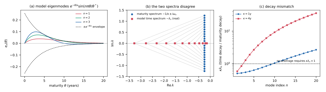
![Figure 2: (a) Factor autocorrelation on block \(n=2\) ( \(\kappa =4\) , \(\theta ^*=30\) ): the arbitrage-free dynamics \(e^{M_n^\top h}\) spirals (decay \(1/\kappa \) , rotation \(\omega _n\) ), the model’s \(e^{-\lambda _nh}\) decays along a ray. This is Corollary 4.5 in a picture. (b) The
completion’s convexity: partial sums \(q^N\) against the exact limit \(\frac {\sigma _0^2}2e^{-2\tau /\kappa }\) ; every \(q^N\) vanishes at \(\tau =0\) while the
limit jumps to \(\sigma _0^2/2\) ; the Gibbs layer narrows as \(\theta ^*/N\) . The layer has the universal profile \(\sigma _0^2\,G(N\pi \tau /\theta ^*)\) , \(G(u)=\frac 2\pi [\Si (u)-\tfrac 12\Si (2u)]\) , with
reinforced first-layer peak \(1.455\times \sigma _0^2/2\) near \(\tau =\theta ^*/N\) (Theorem 5.2 ). (c) The two arbitrage-free completions of
Remark 5.3 (iii).](figs/fig2.svg)